Control System Design Based on Frequency Response Analysis
Frequency response concepts and techniques play an important role in control system design and analysis. Control System Design Based on Frequency Response Analysis. Closed-Loop Behavior. In general, a feedback control system should satisfy the following design objectives:.


Control System Design Based on Frequency Response Analysis
E N D
Presentation Transcript
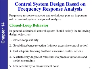
Frequency response concepts and techniques play an important role in control system design and analysis. • Control System Design Based on Frequency Response Analysis Closed-Loop Behavior In general, a feedback control system should satisfy the following design objectives: • Closed-loop stability • Good disturbance rejection (without excessive control action) • Fast set-point tracking (without excessive control action) • A satisfactory degree of robustness to process variations and model uncertainty • Low sensitivity to measurement noise
Controller Design Using Frequency Response Criteria Advantages of FR Analysis: 1. Applicable to dynamic model of any order (including non-polynomials). 2. Designer can specify desired closed-loop response characteristics. 3. Information on stability and sensitivity/robustness is provided. Disadvantage: The approach tends to be iterative and hence time-consuming -- interactive computer graphics desirable (MATLAB) Chapter 14
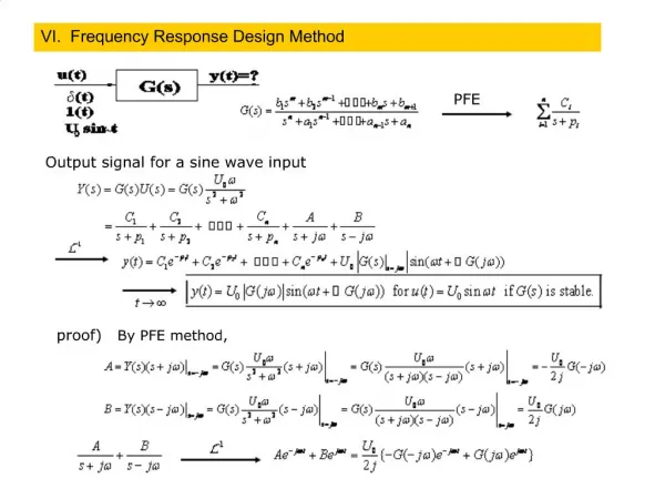
Complex Variable Z-P=N Theorem If a complex function F(s) has Z zeros and P poles inside a certain area of the s plane, the number of encirclements (N) a mapping of a closed contour around the area makes in the F plane around the origin is equal to Z-P.
Dynamic Behavior of Closed-Loop Control Systems 4-20 mA Chapter 11
Important Conclusion The C+ contour, i.e., Nyquist plot, is the only one we need to determine the system stability!
General Stability Criterion A feedback control system is stable if and only if all roots of the characteristic equation lie to the left of the imaginary axis in the complex plane.
Advantages of Bode Stability Criterion The Bode stability criterion has two important advantages in comparison with the Routh stability criterion of Chapter 11: • It provides exact results for processes with time delays, while the Routh stability criterion provides only approximate results due to the polynomial approximation that must be substituted for the time delay. • The Bode stability criterion provides a measure of the relative stability rather than merely a yes or no answer to the question, “Is the closed-loop system stable?”
Example 14.3 A process has the third-order transfer function (time constant in minutes), Also, Gv= 0.1 and Gm= 10. For a proportional controller, evaluate the stability of the closed-loop control system using the Bode stability criterion and three values of Kc:1, 4, and 20. Solution For this example,
Figure 14.5 shows a Bode plot of GOLfor three values of Kc. Note that all three cases have the same phase angle plot because the phase lag of a proportional controller is zero for Kc> 0. Next, we consider the amplitude ratio AROLfor each value of Kc. Based on Fig. 14.5, we make the following classifications:
In Section 12.5.1 the concept of the ultimate gain was introduced. For proportional-only control, the ultimate gain Kcu was defined to be the largest value of Kc that results in a stable closed-loop system. The value of Kcu can be determined graphically from a Bode plot for transfer function G = GvGpGm. For proportional-only control, GOL= KcG.Because a proportional controller has zero phase lag if Kc > 0, ωc is determined solely by G. Also, AROL(ω)=Kc ARG(ω) (14-9) where ARG denotes the amplitude ratio of G. At the stability limit, ω= ωc, AROL(ωc) = 1 and Kc= Kcu. Substituting these expressions into (14-9) and solving for Kcu gives an important result: The stability limit for Kc can also be calculated for PI and PID controllers, as demonstrated by Example 14.4.
For many control problems, there is only a single and a single . But multiple values can occur, as shown in Fig. 14.3 for . Figure 14.3 Bode plot exhibiting multiple critical frequencies.
Important Properties of the Nyquist Stability Criterion • A negative value of N indicates that the -1 point is encircled in the opposite direction (counter-clockwise). This situation implies that each countercurrent encirclement can stabilize one unstable pole of the open-loop system. • Unlike the Bode stability criterion, the Nyquist stability criterion is applicable to open-loop unstable processes. • Unlike the Bode stability criterion, the Nyquist stability criterion can be applied when multiple values of critical frequencies or gain cross-over ferquencies occur.
Example Evaluate the stability of the closed-loop system for: Gv= 2, Gm= 0.25, Gc = Kc Obtain ωc and Kcufrom a Bode plot. Let Kc =1.5Kcu and draw the Nyquist plot for the resulting open-loop system.
Solution The Bode plot for GOL and Kc = 1 is shown in Figure 14.7. For ωc = 1.69 rad/min, OL= -180° and AROL = 0.235. For Kc = 1, AROL = ARG and Kcucan be calculated from Eq. 14-10. Thus, Kcu = 1/0.235 = 4.25. Setting Kc = 1.5Kcugives Kc = 6.38. Figure 14.7 Bode plot for Example 14.6, Kc = 1.
Figure 14.8 Nyquist plot for Example 14.6, Kc = 1.5Kcu = 6.38.