3-location Data Network Design
This project involves designing a data network for 3 locations separated by 200 km, catering to specific user populations and traffic patterns, considering email, web, and database traffic along with server distribution and network principles.

3-location Data Network Design
E N D
Presentation Transcript
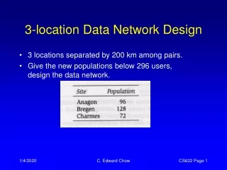
3-location Data Network Design • 3 locations separated by 200 km among pairs. • Give the new populations below 296 users, design the data network. C. Edward Chow
Voice Traffic vs. Data Traffic C. Edward Chow
Data Traffic Statistics • 20% of internal email, www, DB traffic occurs in the busy hour. • External email arrives evenly during the day. • Avg. internal email size 60kB. External email size 12kB. • Each url request generates 6 datagrams to server, 6 datagrams back to client for setup connections, a datagram avg. 128B. • Its http response is 2kB datagram. C. Edward Chow
Data Base Traffic • Data distributed in 3 servers, one at each site. • Each employee makes 100 queries and 5 updates. • Query: • Query first goes to the local server, then go the remote server. Will there need to go to third server? • Query packet avg. 800B, response packet avg. 3500B. • Probability of data in a server is 1/3. Evenly spread. • Update: • Update packet avg. 6000B, response packet 500B. C. Edward Chow
Cost of Services and Components Cost of PC’s, workstations, servers not considered. Routers can handle 2000 datagrams/sec >> the traffic Delay can be neglected. C. Edward Chow
Data Network Design Principle 2.2 • Blocking in not important; delay is the issue. • Highly utilized links are not desirable (large delay). Design Principle 2.2 • In a voice network, highly utilized links can be cost-effective, since they exploit the available bandwidth to the fullest extent, and when the link is given to a connection it receives a high grade of service (circuit switch). • In a data network, highly utilized links are terrible since all call traffic using that link suffers inordinate delay. C. Edward Chow
Burstiness • Burstiness= peak rate/avg rate Two solutions to simultaneous arrive of data calls: • Coordination- e.g., token ring. Allow one to be servered. But is not good for WAN.Propagation delay (p.d.) for 1000 mile ring=1000/186000=5msTransmission delay for 1000 bit packet at 16Mbps=1000/16000000 << p.d. • Queueing or use store and forward (packet switching idea). C. Edward Chow
Common Data Rate The service time for a packet of n bits on a link of speed S bps is n/S C. Edward Chow
Token Ring vs. Packet Switching Propagation delay for 1000 mile ring=1000/186,000=5.376 ms Transmission delay for 1000 bit packet at 16Mbps=1000/16,000,000 =0.0625ms For WAN, token ring protocol is not suitable. A packet switching network where each link segement operates independently is a more efficient design. Packet switching network can be modeled as a set of queues. C. Edward Chow
M/M/1 Queue • Link can be modeled as a M/M/1 queue. C. Edward Chow
M/M/1 Average Waiting Time C. Edward Chow
Total Delay (50ms service time) C. Edward Chow
Initial Data Network Design C. Edward Chow
Cost of Initial Design • Transit router amortized cost: $3700*0.03=$111/month • 64kbps (or D64) internode link $700/month • 64kbps internet link $1400/month. C. Edward Chow
Traffic in Busy Hour • 20%=0.2 traffic in busy hour. C. Edward Chow
Design Principles 2.3 & 2.4 2.3: Seek to make a network where all the links have a 50% utilization 2.4: Seek to make a network where all the links have about 50% utilization and as few links as possible are underutilized. Example: Question1: How we calculate the delay? Question2: For high speed link, can we have high utilization? C. Edward Chow
Apply M/M/1 Formula • Assume 1000 bytes packet (8000 bits). • Case1: T1 link=1.536Mbps, 50% utilization • Case2: OC-3 link=135Mbps, 80% utilization • Which one has lower delay? C. Edward Chow
Apply M/M/1 Formula Case1: T1 link=1,536,000 bps, r=0.5 (50%utilization) • 1/m= service time=packetsize/transmission speed=8000/1536000 • T=(1/m)/(1-r)=(1/(1-r))*(1/m)=(1/(1-0.5))*8000/1.536M=10.4 ms. Case2: OC-3 link=135Mbps, r=0.8 (80% utilization) • T=(1/(1-0.8))*(8000/135M)=5*(8000/135M)=2.96ms • We may be willing tolerate a higher utilization on these links. But their delay is quite “unstable”. C. Edward Chow
Calculating Internal Email Traffic • Internal Email: relate to the populations of source and destination sites. The ration of populations among Anagon, Bregen, and Charmes=(1, 4/3, ¾) • Let x be the volume of internal email from Analog to itself. • Then the traffic from Anagon to Bregen is 4/3 x. • The traffic from Anagon to Charmes is ¾ x. • busy hour internal email: 10*0.2*60000*8*296/3600(s)=78933 bps. • Counting all directional internal email traffic: 9.507x=78933bps x=8303bps C. Edward Chow
Tabular Represenation of Internal Email Traffic C. Edward Chow
External Email • In the initial design, each site has its own Internet connection. Therefore the external emails does not go through inter-site internal network. • Internet links are expensive: first targets to remove;then external emails could go over inter-site network. • With 4000 emails/day, 12000 B/emaileach user gets 4000*12000*8/(3600*8hr*296)=45.045bpssends same 45.045bps external emails. • Multiply the population in each site we get the following external traffic table. C. Edward Chow
Tabular Represenation of External Email Traffic • 45.045*96=4324.32 bps C. Edward Chow
Busy Hour WWW Traffic • Outbound small requests traffic: =40fetch/day*0.2*6req/fetch*128B/req*8b/B/(3600s)=13.653bps • Inbound big www document and response traffic:=40*0.2*(6x128+2000)*8/(3600)=49.209bps • For Anagon, Inbound WWW traffic: 13.653bps*96=1310.72bpsoutbound WWW traffic:49.209bps*96=4724.05bps C. Edward Chow
Busy Hour WWW Traffic C. Edward Chow
DB Query Flow • Assume query can be answered by a single remote server. C. Edward Chow
Busy Hour DB Traffic DB Query Traffic: • 1/3 queries to each remote server:50*0.2*800*8*(1/3)/3600=5.930 bps • Their requests come back:50*0.2*3500*8*(1/3)/3600=25.926bps DB Update Traffic: • 1/3 updates to each remote server:5*0.2*6000*8*(1/3)/3600=4.444 bps • 1/3 updates responses back from each remote server:5*0.2*500*8*(1/3)/3600=0.370 bps DB Traffic From Anagon to Bregen: • Consider just DB Query(text): 96*5.930+128*25.926=3887.8 • Consider all DB traffic: The update traffic should not be ignored 96*(5.930+4.444)+128*(25.926+0.370)=4357.568 C. Edward Chow
DB Traffic Table C. Edward Chow
Busy Hour Traffic (64kbps links) C. Edward Chow
Busy Hour Traffic C. Edward Chow
Drop Algorithm for Network Design • Drop the lightest utilized component in the network. • Calculate the new routes for all traffic that use the dropped component. • But do we really have control over the routing in the network? • We will examine 3 types of routing: • SNA (IBM System Network Architecture) tight control • OPSF (Open Shortest Path First) some control • RIP (Routing Information Protocol) no control C. Edward Chow
Routing in SNA • On IBM SNA (System Network Architecture), designer has up to 16 routes that can be specified between a pair of nodes. The paths are directional. The return path of a route can go through different links. • Advantage: flexible, a lot of control • Disadvantage: adding a node is not automatic, required offline programs to generate the paths. C. Edward Chow
OPSF Routing • Assign each link a length (or weight) in each direction. • Routes are calculated using shortest path algorithm. • Traffic are directed to the next link along the shortest path. • Two routes between a pair of nodes. (compared to max. of 16 for SNA) • Weight can be measured as delay on the directional link. • Link weights can be broadcast periodically and routing table recalculated. C. Edward Chow
Routing Information Protocol • Use hop count instead of accumulated link weight for compute the route. • Does not consider the bandwidth of each link. • For 1000-byte packet, • a two hop path with T1 link has(1000*8b/1.535Mbps)*2=10.42ms. • A single hop path with 9.6kbps link has1000*8b/9600bps=833ms. C. Edward Chow
Assumptions for Drop Algorithm • Assume we can use shortest path routing within BMI corp. domain. • All three inter-site links have a length of 10. • The distance to all external domains is the same through all three gateways. • Try to reduce cost by removing links and see if remaining network remain feasible. C. Edward Chow
Drop Algorithm • Initially, mark all links as being deletable. • Find the most expensive deletable link. If there is a tie, take the link with the lowest utilization. We call this the candidate link for deletion. • If such link exists, delete the link and see if the remaining network is feasible (can carry the traffic). • If it is feasible, go back to step 2. • If not feasible, mark the link “not being deletable” and loop back to step 2. • If such link does not exist, terminate. C. Edward Chow
Modified Drop Algorithm Code Consider increase other link’s capacity C. Edward Chow
Apply Drop Algorithm on Initial Design Round 1. • Step2. Among 3 external links, choose Charmes to gateC. • Step3’. Redirect traffic to Gateway A (with less traffic)by reducing the length btw Anagon and Charmes to 9. • GateCCharmes traffic (WWW+External Email) go over GateAAnagonCharmes. • CharmesGateC traffic go over CharmesAnagonGateA • The new traffic flow is shown next page. C. Edward Chow
Traffic Flow After Removing Link to GateC All link utilizations < 0.5; cost saving=$1400 C. Edward Chow
Apply Drop Algorithm on Initial Design Round 2. • Step2. Among 2 external links, choose Bregen to gateB since it has less traffic now. • Step3’. Redirect traffic to Gateway A (with less traffic) • GateBBregen traffic (WWW+External Email) go over GateAAnagonBregen. • BregenGateB traffic go over BregenAnagonGateA • The new traffic flow is shown next page. C. Edward Chow
Traffic Flow After Removing Link To GateB • All link utilizations < 0.5; cost saving another $1400 C. Edward Chow
Round 3 & Round 4 • Round 3: Try to delete link to gateA and find it undeletable. • Round 4: Among the remaining 3 inter-site links, BregenCharmes has less utilization (add both directional traffic). • Redirect traffic around Anagon. C. Edward Chow
Traffic Flow After Removing Link btw Bregen and Charmes • Utilization between Anagon and Bregen high, need add link? C. Edward Chow
Rounds 4, 5, 6 • After removing link btw Charmes and Bregen, we need to add capacity to Anagon and Bregen no cost saving. • We also lose alternative route (less reliability). • Decide not to remove. • Same results for link btw Anagon and Charmes, and link between Anagon to Bregen. • Algorithm terminates. C. Edward Chow
Drop Algorithm Result • 2 internet links removed cost saving $2800/month C. Edward Chow
Where the Drop Algorithm Went Wrong? • It chooses Anagon instead of Bregen, which has most traffic and largest population. • This force more traffic onto longer paths. • Lesson: Heuristic algorithms often make mistakes. • If we choose to locate gateway at Bregen, we could remove link btw Anagon and Charmes: • Save $700/month • Save $102/month by placing terminal routers at Anagon and Charmes. • Final cost: $3833-$700-$102=3031/month. C. Edward Chow
Final Design Definition 2.3: A benign algorithm is one that does no damage to a design. It only improve it or leave it alone. The drop algorithm is not optimal but is it benign? C. Edward Chow
Homework #5 A B C D • Exercise 2.6. Assume the traffic in Table 2.17 increases 5 times. Design a low-cost solution for the BMI Corporation. • Exercise 2.8. In figure 2.17, we have a 4-site network.Given the traffic matrix, use the drop algorithm to redesign the network. Each link is limited to 28,000bps in each direction. Further assume that each link costs $100 times the length of the link. AD link is $100*100. A B C D C. Edward Chow
Solution to Hw#5 Exercise 2.6. 5 times the original Busy Hour Traffic: C. Edward Chow
Exercise 2.6 • Traffic between sites > 32kbps can not use single 64kbps lines at a 50% utilization (design goal/principle). • According to the pricing info. It does not pay to have two 64kbps lines. We should go for the 256kbps line (same price!) C. Edward Chow
Exercise 2.6 • For Internet links, we need to go for 256kbps too. • Actually the total incoming Internet traffic is 139375bps and requires two 256kbps lines to be lower than the 50% utilization. • We locate the two Internet links at Anagon and Bregen since Charmes’ traffic is the smallest. • Charmes’ Internet traffic needs to be rerouted. Since Anagon has lower utilization, it was routed to Anagon. • AnagonCharmes traffic increases by 33930bps. • CharmesAnagon traffic increases by 21130bps. C. Edward Chow