Download

1 / 81
810 likes | 1.03k Vues
Clustering and Shifting of Regional Appearance for Deformable Model Segmentation. Joshua V. Stough. MIDAG, UNC-Chapel Hill July 25, 2008. Radiation Therapy Planning for Prostate Cancer. Goal : Treat prostate while avoiding neighboring tissue. Requires Segmentation Problems :

E N D
Clustering and Shifting of Regional Appearance for Deformable Model Segmentation Joshua V. Stough MIDAG, UNC-Chapel Hill July 25, 2008
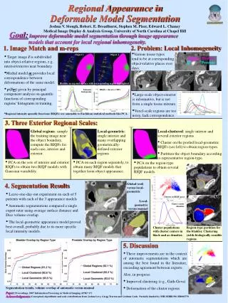
Radiation Therapy Planning for Prostate Cancer • Goal: Treat prostate while avoiding neighboring tissue. • Requires Segmentation • Problems: • Low contrast • High variability • Result: Segmentation is challenging and high cost for clinicians.
Automating Segmentation Using Deformable Models • Automatically deform an object model to fit the image data. • Bayesian DMS • Requires an object model and a measure of image fit – image match.
M-rep Deformable Model • M-rep provides: • Boundary rep. with normals • Statistical deformation p(m) • Correspondence • Locality [Pizer et al., IJCV 55 (2) 2003][Fletcher et al., TMI 23 (8) 2004]
Image Match p(I | m): Related Work • Profile-based, voxel-scale correspondence • AAM, [Cootes et al., CVIU 61 (1) 1995] • AAM +, [Scott et al., IPMI 2003] • Intensity Profile Clustering, [Stough et al., ISBI 2004] • Region-based • Intensity Ranges, [Zhu et al., PAMI 18 (9) 1996] • Summary Statistics • [Tsai et al., TMI 22 (2) 2003] • [Chan et al., TIP 10 (2) 2001] • Histogram Metrics • [Rubner et al., CVIU 84 2001] • [Freedman et al., TMI 24 (3) 2005] • Statistics on Distributions, [Broadhurst, UNC 2008]
Appearance: Regional Intensity Quantile Functions (RIQFs) • Example – global object-relative regions. [Credit: Eli Broadhurst] • Principal component analysis (PCA)
Correspondence in Regional Image Matches Key is correspondence, both geometry- and image-based. Two factors: m-rep induced actual differences inorgan relationships • Result: the geometric correspondence given is weakly related to the image correspondence desired. • Clustering to find regions. Shifting to account for their motion.
Goal: Improved Segmentation Through Image Match Thesis:Segmentation benefits from the use of object-relative, regional statistical appearance models. Specifically, Clustering provides an effective understanding of the context of the object of interest in the image. Shifting of appearance allows for relaxation of the geometric correspondence.
Question: Which Image Match Produces Best Segmentations? Global regions Versus geometrically defined local regions Versus regions defined by RIQF clusters.
Determine Region Types • Pool RIQFs over all regions and training images. • Gath-Geva Clustering • Example: C= 4 on bladder exterior. [Gath, Geva PAMI 11 (7) 1989]
Characterize the Appearance of the Larger-Scale Regions • For each local region, choose most popular cluster. • Combine local regions belonging to the same cluster. • PCA on the larger-scale regions. • PCA over all training images
Experimental Setup Determine local RIQF-types in training data. Construct Gaussian models on the regions represented by the cluster types. Build a template of optimal types. • 5 patient image sets, ~16 images per patient. • UNC RadOnc and William Beaumont, Michigan. • 512 5120.98 0.98 3 mm • Volume Overlap, Average Surface Distance, Maximum Distance
Results • Clustered regional image match led to improved segmentations over global. • For this study: approaching expert quality, exceeding agreements between experts
Motivation: Shifting • Geometric correspondence is not image correspondence.
Allegiance-based Shifting • Each point and its RIQF on the surface is assigned a region. • Larger-scale RIQF is formed by combining the RIQFs of all points with that allegiance. • A point can change allegiance if: • On boundary • Exclusion from current region benefits current region • Addition to prospective region benefits prospective region • Or: change is a net benefit
Clustered Shifting • Initialize at modal allegiance • Iterate over points on boundary, change allegiance if appropriate
Example of Clustered Shifting Before: After:
Local Shifting • Subdivision of local regions • Additional connectivity constraints
Results • Shifting is better than static in bladders, not in prostates. • All image matches: Overall quality approaching clinical in this study.
Conclusions • Clustering leads to effective appearance models for DMS. • Shifting can account for the variability in the external conformation of neighboring regions.
Future Directions • Applications • hippocampus, caudate and other subcortical structures in MRI • Reformulation of shifting (warp or contours) • Tissue Mixture Modeling
Thank you. • Committee • MIDAG • Department staff • Teaching opportunities • Mia
Outline • Medical Image Segmentation • Computed tomography • Bayesian deformable model segmentation • Appearance models and image match • Thesis • Novel appearance models, results • Conclusions
Computed Tomography • Diagnosis • Radiation Therapy Planning (RTP) • Image-guided surgery • Shape analysis…
M-rep Deformable Model • M-rep provides: • Boundary rep. with normals • Statistical deformation p(m) • Correspondence • Locality [Pizer et al., IJCV 55 (2) 2003][Fletcher et al., TMI 23 (8) 2004]
Image Match p(I | m): Related Work • Profile-based, voxel-scale correspondence • AAM, [Cootes et al., CVIU 61 (1) 1995] • AAM +, [Scott et al., IPMI 2003] • Intensity Profile Clustering, [Stough et al., ISBI 2004] • Region-based
Profile Appearance • Relative object position affects intensity pattern. • Local profile types. • grey-to-light, grey-to-dark, notch Axial CT slice Coronal CT slice IN OUT
Template Best Describes Dominant Intensity Pattern in the Boundary Region Outside Inside Left kidney Right kidney
Bladder and Prostate in CT • Profiles are unstable, discount spatial coherence. • Think regional.
Image Match p(I | m): Related Work • Profile-based, voxel-scale correspondence • AAM, [Cootes et al., CVIU 61 (1) 1995] • AAM +, [Scott et al., IPMI 2003] • Intensity Profile Clustering, [Stough et al., ISBI 2004] • Region-based • Intensity Ranges, [Zhu et al., PAMI 18 (9) 1996] • Summary Statistics • [Tsai et al., TMI 22 (2) 2003] • [Chan et al., TIP 10 (2) 2001] • Histogram Metrics • [Rubner et al., CVIU 84 2001] • [Freedman et al., TMI 24 (3) 2005] • Statistics on Distributions, [Broadhurst, UNC 2008]
Appearance: Regional Intensity Quantile Functions (RIQFs) • Example – global object-relative regions. [Credit: Eli Broadhurst] • Example – PCA.
Previous Regional Techniques • Deficiencies • Global discounts context • Summary statistics ignore nuance • Solution: regional, QF-based statistical image match • Region: organ or other volume whose local intensity distributions are distinguishable from those of neighboring volumes.
Thesis Segmentation benefits from the use of object-relative, regional statistical appearance models. Specifically, Clustering on object-relative image descriptors Shifting to relax geometric correspondence
Outline • Medical Image Segmentation • Thesis • Novel appearance models, results • Clustering and Appearance at Regional Scale • Shifting Regional Appearance • Conclusions
Question: Which Image Match Produces Best Segmentations? Global regions Versus geometrically defined local regions Versus regions defined by RIQF clusters.
Determine Region Types • Pool RIQFs over all regions and training images. • Gath-Geva Clustering • Example: C= 4 on bladder exterior. [Gath, Geva PAMI 11 (7) 1989]
Partition the Boundary by Cluster Type • For each local region, choose most popular cluster. • Combine local regions belonging to the same cluster.
PCA on larger-scale RIQFs • Combine local RIQFs through interpolation in the CDF space. • PCA over all training images
Experimental Setup Determine local RIQF-types in training data. Construct Gaussian models on the regions represented by the cluster types. Build a template of optimal types. • 5 patient image sets, ~16 images per patient. • UNC RadOnc and William Beaumont, Michigan. • 512 5120.98 0.98 3 mm • Dice Similarity Coefficient, Average Surface Distance
Results, Global v Local v Clustered RIQF clustered image match compares favorably with global, not as good as local
Results, Global v Local v Clustered RIQF clustered image match compares favorably with global, not as good as local
Results • Hausdorff medians • Images • Good improvement • Bad improvement
Outline • Medical Image Segmentation • Thesis • Novel appearance models, results • Clustering and Appearance at Regional Scale • Shifting Regional Appearance • Conclusions
Motivation: Shifting • Geometric correspondence is not image correspondence.
Allegiance-based Shifting • Each point and its RIQF on the surface is assigned a region. • Larger-scale RIQF is formed by combining the RIQFs of all points with that allegiance. • A point can change allegiance if: • On boundary • Exclusion from current region benefits current region • Addition to prospective region benefits prospective region