Multiview stereo
Multiview stereo. Volumetric stereo. Scene Volume V. Input Images (Calibrated). Goal: Determine occupancy, “color” of points in V. Discrete formulation: Voxel coloring. Discretized Scene Volume. Input Images (Calibrated). Goal: Assign RGBA values to voxels in V
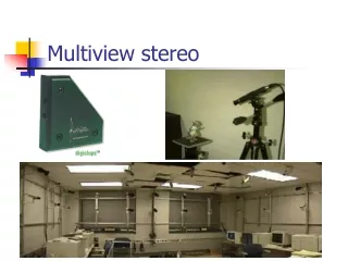

Multiview stereo
E N D
Presentation Transcript
Volumetric stereo Scene Volume V Input Images (Calibrated) Goal: Determine occupancy, “color” of points in V
Discrete formulation: Voxel coloring Discretized Scene Volume Input Images (Calibrated) • Goal: Assign RGBA values to voxels in V • photo-consistent with images
True Scene All Scenes (CN3) Photo-Consistent Scenes Complexity and computability Discretized Scene Volume 3 N voxels C colors
1. Choose voxel • Color if consistent • (standard deviation of pixel • colors below threshold) 2. Project and correlate Voxel coloring Visibility Problem: in which images is each voxel visible?
Layers Depth ordering: occluders first! Scene Traversal Condition: depth order is the same for all input views
Panoramic Depth Ordering • Cameras oriented in many different directions • Planar depth ordering does not apply
Inward-Looking • cameras above scene • Outward-Looking • cameras inside scene Compatible Camera Configurations
Voxel Coloring Results Dinosaur Reconstruction 72 K voxels colored 7.6 M voxels tested 7 min. to compute on a 250MHz SGI Flower Reconstruction 70 K voxels colored 7.6 M voxels tested 7 min. to compute on a 250MHz SGI
A view-independent depth order may not exist Limitations of Depth Ordering p q • Need more powerful general-case algorithms • Unconstrained camera positions • Unconstrained scene geometry/topology
Initialize to a volume V containing the true scene • Choose a voxel on the current surface • Project to visible input images • Carve if not photo-consistent • Repeat until convergence Space Carving Algorithm Image 1 Image N …...
p Convergence • Consistency Property • The resulting shape is photo-consistent • all inconsistent points are removed • Convergence Property • Carving converges to a non-empty shape • a point on the true scene is never removed
V Photo Hull Which shape do you get? V • The Photo Hull is the UNION of all photo-consistent scenes in V • It is a photo-consistent scene reconstruction • Tightest possible bound on the true scene True Scene
Space Carving Results: African Violet Input Image (1 of 45) Reconstruction Reconstruction Reconstruction
Space Carving Results: Hand Input Image (1 of 100) Views of Reconstruction
Comparison with stereo • Much harder problem than stereo • In stereo, most scene elements are visible in both cameras • It is common to ignore occlusions • Here, almost no scene elements are visible in all cameras • Visibility reasoning is vital
Key issues • Visibility reasoning • Incorporating spatial smoothness • Computational tractability • Only certain energy functions can be minimized using graph cuts! • Handle a large class of camera configurations • Treat input images symmetrically
Approach • Problem formulation • Discrete labels, not voxels • Carefully constructed energy function • Minimizing the energy via graph cuts • Local minimum in a strong sense • Use the regularity construction • Experimental results • Strong preliminary results
Problem formulation • Discrete set of labels corresponding to different depths • For example, from a single camera • Camera pixel plus label = 3D point • Goal: find the best configuration • Labeling for each pixel in each camera • Minimize an energy function over configurations • Finding the exact minimum is NP-hard
q l = 2 l = 3 C1 r p C2 Depth labels Sample configuration
Energy function has 3 terms: smoothness, data, visibility • Neighborhood systems involve 3D points • Smoothness: spatial coherence (within camera) • Data: photoconsistency (between cameras) • Two pixels looking at the same scene point should see similar intensities • Visibility: prohibit certain configurations (between cameras) • A pixel in one camera can have its view blocked by a scene element visible from another camera
l = 2 l = 3 p C1 r Smoothness neighbors Depth labels Smoothness neighborhood
Smoothness term • Smoothness neighborhood involves pairs of 3D points from the same camera • We’ll assume it only depends on a pair of labels for neighboring pixels • Usual 4- or 8-connected system among pixels • Smoothness penalty for configuration f is • Vmust be a metric, i.e. robustified L1 (regularity)
q l = 2 l = 3 C1 p If this 3D point is visible in both cameras, pixels p and q should have similar intensities C2 Depth labels Photoconsistency constraint
q l = 2 l = 3 C1 p Photoconsistency neighbors C2 Depth labels Photoconsistency neighborhood
Data (photoconsistency) term • Photoconsistency neighborhood Nphoto • Arbitrary set of pairs of 3D points (same depth) • Current implementation: if the projection of on C2 is nearest to q • Our data penalty for configuration f is • Negative for technical reasons (regularity)
q l = 2 l = 3 C1 p is an impossible configuration C2 Depth labels Visibility constraint
q l = 2 l = 3 C1 p Visibility neighbors C2 Depth labels Visibility neighborhood
Visibility term • Visibility neighborhood Nvis is all pairs of 3D points that violate the visibility constraint • Arbitrary set of pairs of points at different depths • Needed for regularity • The pair of points come from different cameras • Current implementation: based on the photoconsistency neighborhood • A configuration containing any pair of 3D points in the visibility neighborhood has infinite cost
Input (non-binary) f Input (non-binary) f Red expansion move C2 C1 Energy minimization via expansion move algorithm • We must solve the binary energy minimization problem of finding the -expansion move that most reduces E • We only need to show that all the terms in E are regular!
Smoothness term is regular • True because V is a metric
Visibility term is regular • Consider a pair of pixels p,q • Input configuration has finite cost • Therefore A=0 • 3D points at the same depth are not in visibility neighborhood Nvis • Therefore D=0 • B,C can be 0 or , hence non-negative
Tsukuba images Our results, 4 interactions
Comparison Best results [SS ’02] Our results, 10 interactions