Download
1 / 24
240 likes | 399 Vues
Chaos Control in a Transmission Line Model. Dr. Ioana Triandaf Nonlinear Dynamical Systems Section Code 6792 Naval Research Laboratory Washington, DC 20375 Ioana.triandaf@nrl.navy.mil IEEE International Conference on Electronics,Circuits and Systems,

E N D
Chaos Control in a Transmission Line Model Dr. Ioana Triandaf Nonlinear Dynamical Systems Section Code 6792 Naval Research Laboratory Washington, DC 20375 Ioana.triandaf@nrl.navy.mil IEEE International Conference on Electronics,Circuits and Systems, December 12-15, 2010, Athens, Greece Work supported by Office of Naval Research
Problem and Objective • Problem: Modeling electromagnetic interference: • Analytical and numerical models exist only for simple networks of electronic devices. • Prominence was given to computational methods rather than to the analysis of the • qualitative behavior of the solutions. • Many open questions remain in the area of relating field tests to current theory for the • analysis, design, and control of dynamically interacting nonlinear networks. • Understanding failure mechanisms in such networks is highly relevant to defense as well • as commercial applications. • Objective: Predict disruption and damage in electronic devices • Obtain a qualitative analysis of solutions of circuit networks over a wide parameter space. • Understanding at a fundamental level of how the transition to damage occurs • Our intention is to understand the underlying dynamics, forecast future effects, and control effects.
Talk Outline • Statement of the problem and motivation • Present the broad research goal • Transmission line equations and properties • Chaotic dynamics in an infinite-dimensional electromagnetic system • Control of the chaotic behavior
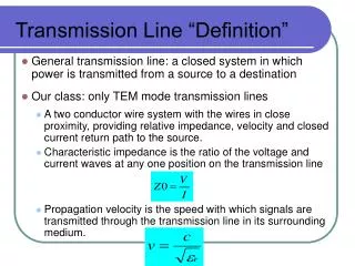
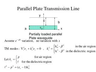
The Dynamic Equations of Transmission Lines Approach: assume that the transverse electric and magnetic fields surrounding the conductor is transverse to the conductor (the quasi-TEM approximation), these are dominant modes when the cross-sectional dimensions of the guiding structure are less than the smallest characteristic wavelength of the electromagnetic field propagating along it. Ideal transmission lines: ideal guiding structures, model interconnections without losses, uniform in space and with parameters independent of frequency. The equations for the voltage and current distribution are: where L is the inductance per-unit-length and C is the capacitance per-unit-length. Sketch of a two-conductor transmission line
Lossy Transmission Lines with Distributed Sources Lossy transmission lines: R the per-unit-length resistance and G the per-unit-length conductance Transmission lines with distributed sources: The distributed sources depend on the incident electromagnetic field and on the structure of the guiding system modeled by the transmission line.
D’Alembert Solution of Two-Conductor Transmission Lines Equations The general solution of the line equation in d’Alembert form is: is the forward voltage wave, is the backward voltage wave This solution can be represented in terms of forward and backward voltage waves only, we can also represent it through the superposition of forward and backward current waves and are univocally determined by the initial conditions: for (an infinite line) for
We consider the case in which the semi-infinite line is connected to a nonlinear resistor: Impose that the solution satisfies , g is the characteristic of the resistor. The equation for is: There may be multiple solution depending on the characteristic curve of the resistor. The Case of a Semi-infinite Line Connected to a Nonlinear resistor
We consider the case in which the semi-infinite line is connected to a nonlinear resistor connected in parallel to a linear capacitor. The equivalent circuit is illustrated as: The equation for is: this equation must be solved together with the initial condition for . Because of the presence of the capacitor the relation between and is no longer of the instantaneous type, but is of the functional type, with memory. Difficulties will proliferate as we consider more and more complex circuital elements. A Semi-infinite Line Connected to a Nonlinear Resistor in Parallel to a Capacitor
Chaotic Dynamics in an Infinite-Dimensional Electromagnetic System Bifurcation and chaos phenomena theoretically observed in a simple electromagnetic system consisting of a linear resistor and a pn-junction diode connected by a transmission line: The system is infinite-dimensional because of the presence of the transmission line and the nonlinearity arises due to the pn-junction diode. We solve the above equation obeying initial conditions , and nonlinear boundary conditions: L. Corti, L. De Menna, G. Miano and L. Verolino, IEEE Trans on Circuits and Systems, Vol. 41, No. 11, November 1994
Solving the Transmission Line Initial Boundary Value Problem By imposing initial conditions and to the general solution for : we obtain for : By imposing the voltages and currents at line ends, , and , we obtain the relation between the state of the line and the electrical variables at the line ends, for in implicit form: The relationship between the value of the backward wave at a boundary point and the value of this wave at a point inside the spatial domain is given by:
Formulation of the Problem as a Dynamical System The general solution of the Telegrapher’s equation is: By imposing boundary conditions: we obtain the nonlinear implicit functional equation: We are making it explicit in the form:
Formulation of the Problem as a Dynamical System The equation provides a convenient way to compute the forward travelling wave at the point and at time when its value at time is known. We formulate the functional equation as a recurrence relation in which the time is discretized obtaining: The dynamic of the voltage at and at is given by:
The pn-junction Diode Dynamics We investigate the system with a pn-junction diode defined by the constitutive equation: where is the saturation current and the thermal voltage. The maximum of the function F is reached when the incremental resistance of the diode is equal to the characteristic impedance. In this case the Poincare map: becomes:
Chaotic Dynamics of the System If the linear resistor is active , oscillations and chaotic motion appear. We consider corresponding to As increases, a period-doubling cascade of bifurcations forms, leading to chaos. The solution a Spatial profile of the wave at
Control of the Chaotic Dynamics of the System We stabilize a period one orbit of the map , using small fluctuations of the parameter for each spatial point. • “Tracking unstable orbits in experiments” by Schwartz Ira B. and Triandaf Ioana , Phys. Rev. A, vol. 46, number 12, (7439-7444) , Dec 199. • “Tracking sustained chaos: A segmentation method”, by Triandaf, Ioana and Schwartz, Ira B., Phys. Rev. E, vol. 62, number 3, (3529-3534), Sep 2000. • “Tracking unstable steady states: Extending the stability regime of a multimode laser system”, by Gills, Zelda and Iwata, Christina and Roy, Rajarshi and Schwartz, Ira B. and Triandaf, Ioana , Phys. Rev. Lett., vol. 69, number 22, (3169-3172), 1992. • “Quantitative and qualitative characterization of zigzag spatiotemporal chaos in a system of amplitude equations for nematic electroconvection” by Iuliana Oprea, Ioana Triandaf, Gerhard Dangelmayr and Ira B. Schwartz , Chaos 17, 023101 (2007). Spatial profile of the wave at Controlled spatial profile of the wave
Control of the Chaotic Dynamics of the System We stabilize a period one orbit of the map , using small fluctuations of the parameter for each spatial point. The relationship between the value of the forward wave at a boundary point and the value of this wave at a point inside the spatial domain is given by: Spatial profile of the forward at Controlled spatial profile of the wave
The Control Method of the Chaotic Dynamics We stabilize a period one orbit of the map , using small fluctuations of the parameter for each spatial point. The fluctuation in for a given spatial point is given by: , is the fixed point of the map, is the unstable eigenvalue of the fixed point, measures the local drift in the fixed point. The maps used to determine Control parameters over the spatial domain
Control of the Chaotic Dynamics of the System We stabilize a period one orbit of the map , using small fluctuations of the parameter for each spatial point. The relationship between the value of the forward wave at a boundary point and the value of this wave at a point inside the spatial domain is given by: Spatial profile of the wave at Controlled spatial profile of the wave
Control of the Chaotic Dynamics of the System We stabilize a period one orbit of the map , using small fluctuations of the parameter for each spatial point. The relationship between the value of the forward wave at a boundary point and the value of this wave at a point inside the spatial domain is given by: Spatial profile of the wave at Controlled spatial profile of the wave
Summary of our Approach • We considered simple electromagnetic networks modelled by the wave equation with nonlinear boundary conditions. • Objectives: • • Recast the equations as lower dimensional systems, possibly maps. • • Study chaotic behavior of networks. • • Design algorithms that mimick disruption of networks in real devices. • Understand how to solve coupled problems of a profoundly different nature • •Transmission line equationsare linear and time-invariant pde’s of hyperbolic type • • Lumped circuits equations are algebraic ode’s, time-varying and nonlinear • Derive representations that take into account only the terminal behaviour • of the transmission line • •Describe terminal behaviour by linear algebraic difference equations with one delay • •Study the existence and uniqueness of the difference-delay equations or solve in the • multi-valued case • •Explain the occurrence of chaos encountered typically when frequencies increase • beyond 100 MHz
Conclusions • We have presented a chaos control method applied to a simple electromagnetic system. • Control is achieved at times which are integer multiples of the round-trip time of the wave along the transmission line. • The current method will be extended to the full simulation and will provide valuable insight on how to achieve control in that case. • The understanding gained will beused in models derived from basic principles and a full stability analysis of solutions will be performed, leading to a deterministic approach to predict upset and failure of electronic networks. • Gain understanding of disruption in circuits at a fundamental level possibly avoiding intensive computing and data storage required by probabilistic techniques. • Prediction of conditions that lead to upset in electronic device, prediction of pathways to failure in network of circuits.
Radiating Disturbances • Examples of radiated disturbances: • crosstalk between circuits, problems related to printed circuit board, surges produced by switching operations, electrical short produced by a conductor fault in a system. • antenna radiation, lightning or nuclear effects • interconnection between two computer boards • radiation of radio emitters, mobile radio communication, radar interference
Multiconductor Transmission Lines Equations Transmission line having (n+1) conductors: The voltage and the current are vectors, , the per-unit-length self-inductance and , is the per-unit-length self-capacitance. The equations for multiconductor transmission lines
Two-conductor Transmission Lines as Two - Ports Transmission line connecting generic lumped circuits: The general solution of the line equations is: where: . The voltage and current distributions along the line are completely identified by the functions and and viceversa. We consider them as state variables of the line.