Detecting Household Production
Detecting Household Production. Marianne Baxter Boston University and NBER and Dana Rotz Harvard University November 2009. Why is household production important?.

Detecting Household Production
E N D
Presentation Transcript
Detecting Household Production Marianne Baxter Boston University and NBER and Dana Rotz Harvard University November 2009
Why is household production important? Substitution between home and market sectors has been shown to be important for macro aggregates and individual labor supply decisions Of limited use in solving the retirement consumption puzzle? (Rogerson 2009) We do not present a formal model but have in mind the models of Baxter and Jermann (1999), Benhabib, Rogerson and Wright (1991), Greenwood, Rogerson and Wright (1995), McGrattan, Rogerson and Wright (1997) and Rupert, Rogerson, and Wright (2000).
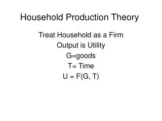
Household production models In these models, households allocate time to market work, home work, and leisure. Substitutions among home goods, market goods and leisure respond to changes in the relative returns to home and market work. Baxter/Jermann (1999) showed that the apparent excess sensitivity of market consumption to predictable changes in market income could be explained by substitution between home and market sectors. Calibrated model with standard parameters.
What data could shed light on this question? Married couples with a single earner have more time available for home production and/or leisure than do married couples with two earners--what are the single-earner families doing with all this extra time? There is a large and growing literature using time-use data. As a complement to these studies… …we ‘detect’ production of home goods and leisure by studying detailed expenditure data, focusing on inputs to home production and leisure
Predictions of household production models Compared with 2-earner households, and controlling for income differences, 1-earner households should: produce more meals at home and purchase fewer meals from restaurants use home capital more intensively (home fuels) spend less on market substitutes for goods that can be produced at home, e.g., housecleaning services spend less on fixed costs of going to work (driving).
Implications for purchases of leisure goods ? In the canonical model, leisure is produced by time alone. In fact, purchases of leisure goods and travel represent about 12% of non-housing after-tax expenditure.
Data: Consumer Expenditure Survey (CEX) Interview survey: Comprehensive expenditure data. Families are in the survey for a maximum of four quarters. Diary survey: One or two weeks for each family. Detailed expenditure data on -- Groceries -- Meals away from home Years covered: 1988-2007 (1982-1987 not used to due to redefinition of key goods)
The Data Married couples, younger than retirement age: --one full-time worker, one 'homemaker' --two full-time workers Of those married individuals not working in the market, 90% are female, and of these 89% state that they are not working 'in order to take care of the home/family'. We drop families with nonworking males since a majority of these are unemployed due to disability (60%). Only 20% claim to be taking care of the home.
Demographic Differences The biggest demographic difference across the family types is in the presence of children, especially young children
Data: Consumer Expenditure Survey (CEX) Of the initial 700+ goods in the interview survey, 400+ goods are related to household production in some way The goods we study represent over 85% of non-housing expenditure These goods were allocated to seven major categories
Major expenditure categories Intermediate inputs to home production (food) Utilization of household capital (fuels) Substitutes for home production (restaurant meals) Fixed costs of going to work (bus fare; suits) General leisure purchases (sporting goods) Travel (airfare) Household capital (purchases of consumer durables; reported value of owned home)
Minor categories, with an example Within each major category are several minor categories, for example: Substitutes for home production -- Food away from home -- Child care -- Home maintenance services—see next slide -- Contractor’s services -- Laundry and dry cleaning, coin-operated -- Alterations and repair of apparel and accessories -- Laundry and dry cleaning, not coin-operated
Individual goods (UCCs) Within each minor categories, there are up to 41 individual UCCs, for example: Substitutes for home production --Home maintenance services -- Service/repair of dishwasher, range hood, etc. -- Fresh flowers or potted plants -- Housekeeping services -- Gardening and lawn care services -- Water softening service -- Services for termite/pest control -- Other repair or maintenance services
The Data We view each family in the sample as an observation on families of a given type. Sometimes families of that type will make a purchase in a given time period and sometimes they will not. By including all families of a given type in the computation of the unconditional expenditure figures, we have a snapshot of what a ‘typical’ family of that type will spend in a ‘typical’ time period.
Structure of Paper Section 2: What are the patterns of expenditure across family types in the raw data? (skip) Section 3: A method for correcting for differences in income and demographic characteristic across family types Section 4: Do we see evidence of home/market substitutions once we correct for income and demographic differences?
Empirical method: overview In the program evaluation literature, a typical question is: “What effect did the job training program have on the trainees’ wages?” To answer this question, trainees are matched with non-trainees with similar characteristics and their wages are compared.
Empirical method: overview, cont’d. Our question is: “What would be the expenditure effect on good j if the family changed from a 2-earner family to a 1-earner family?” We match 1-earner families with ‘similar’ 2-earner families. We compare the expenditure between the single-earner household and its matching two-earner household.
Propensity Score Estimation “Similarity” is defined using the propensity score—the probability that family with two adults has a single earner. The propensity score will depend on: -- The opportunity cost of time spent in home production: Potential income -- Variables that influence home productivity or enjoyment of leisure, including: - Number of children - Age - Race
Summary of econometric procedure Estimate potential income for men and women separately, using characteristics (but not actual income) of both spouses. Estimate the propensity score for each family using potential income of both spouses and other individual and family characteristics, e.g, age of spouses, number of children and ages of children.
Summary of econometric procedure, cont’d. Match each 1-earner family with the 2-earner family with the closest propensity score. We also compared results from matching with up to 5 families. Results not affected. Finally, regress expenditure differences across matched families on income differences and differences in other demographic characteristics. This step is important for adjusting expenditure for income differences between 1-earner and 2-earner families.
Overlap and unconfoundedness There are two statistical conditions on the data that must be satisfied for the method to be appropriate: overlap and unconfoundedness. Bottom line: We’re fine on both counts.
Results Table 8 presents results for the full sample of families, and Children: Families without children Families with a child under 6 years of age Families with a child aged 6-17 Income: Families with low incomes (10th-40th percentile) Families with high incomes (60th-90th percentile) Age: Younger families (average spouse age < 40) Older families (average spouse age > 40)
Table 8: Expenditure Effects of Change from 2 earners to 1 earner Results from Propensity Score Matching Plus Regression (% change from initial 2-earner expenditure level) We expect substitution toward more time-intensive groceries used to produce meals at home, and this is exactly what we find.
Table 8: Expenditure Effects of Change from 2 earners to 1 earner Results from Propensity Score Matching Plus Regression (% change from initial 2-earner expenditure level) Utilization increases across the board; largest for families without children and low-income families.
Table 8: Expenditure Effects of Change from 2 earners to 1 earner (% change from initial 2-earner expenditure level) Market substitutes for home production decrease for all family groups.
Table 8: Expenditure Effects of Change from 2 earners to 1 earner (% change from initial 2-earner expenditure level) Food away from home decreases for all family groups. (Includes take-out.)
Table 8: Expenditure Effects of Change from 2 earners to 1 earner (% change from initial 2-earner expenditure level) Child care expenditures decrease by one-half to two-thirds.
Table 8: Expenditure Effects of Change from 2 earners to 1 earner (% change from initial 2-earner expenditure level) Our most counterintuitive result: Spending on home maintenance services increases, especially families with young children.
Table 8: Expenditure Effects of Change from 2 earners to 1 earner (% change from initial 2-earner expenditure level) No significant effects for contractor’s services—may not be DIY substitutes.
Table 8: Expenditure Effects of Change from 2 earners to 1 earner (% change from initial 2-earner expenditure level) Laundry etc. shows expected pattern: increase for time-intensive coin-operated method, decrease for time-saving alteration and drop-off laundry/dry cleaning.
Table 8: Expenditure Effects of Change from 2 earners to 1 earner (% change from initial 2-earner expenditure level) Total expenditure falls significantly. Decreases in lunch expenditures are about as large as for dinner. Full-service and fast food affected to similar extent.
Table 8: Expenditure Effects of Change from 2 earners to 1 earner (% change from initial 2-earner expenditure level) Leisure: Small overall effect, evidence of substitution toward time-intensive leisure goods Travel: Also small overall, no significant change in time-saving air travel
Table 8: Expenditure Effects of Change from 2 earners to 1 earner (% change from initial 2-earner expenditure level) Women’s clothing expenditures decrease, as expected, but this is not concentrated in work-related items such as suits and uniforms.
Table 8: Expenditure Effects of Change from 2 earners to 1 earner (% change from initial 2-earner expenditure level)
Summary Compared with 2-earner households, we find that 1-earner households: (a) Do produce more meals at home and purchase fewer meals from restaurants. (b) Further, 1-earner households substitute toward high-time-input groceries. Do use home capital more intensively (home fuels, trash, telephone.)
Summary, cont’d. Compared with 2-earner households, we find that 1-earner households: (a) Do spend less on some market substitutes for goods that can be produced at home: restaurant meals and child care, but (b) Do notspend less on housekeeping services or contractor’s services. 4. Do spend less on fixed costs of going to work, notably driving costs and women’s clothing.
Summary, cont’d. Compared with 2-earner households, we find that 1-earner households: (a) Do have different purchase patterns for non-housing home capital: higher furniture purchases, lower new car purchases (b) Do report higher home values 6. Do spend differently on leisure goods, although the aggregate effect is not large. Some evidence that substitution is toward time-intensive goods.
Future Research Is there enough cyclic home/market substitution to explain the consumption ‘excess sensitivity’ puzzle in the way proposed by Baxter/Jermann ? 2. Combine the CEX data with the ATUS data (synthetic cohort analysis) to generate estimates of the home production function(s) 3. This information will be used to formulate and restrict a multi-person model of a household engaged in home work, market work, and the production of leisure


