LINEAR PROGRAMMING
LINEAR PROGRAMMING. YU LIANG CMASS, NCAT. Note:. 3-4 people form a group (A,B,C). Each group turn to answer questions according to dice. Plans for today: Introduction to LP Graphic formulation for LP Resume Gauss-Jordan Standard form of LP Plans for Thursday Simplex Algorithm

LINEAR PROGRAMMING
E N D
Presentation Transcript
LINEAR PROGRAMMING YU LIANG CMASS, NCAT
Note: • 3-4 people form a group (A,B,C). Each group turn to answer questions according to dice. • Plans for today: • Introduction to LP • Graphic formulation for LP • Resume Gauss-Jordan • Standard form of LP • Plans for Thursday • Simplex Algorithm • Advanced topics • Do not take the notes, the slides will be distributed • All questions are welcome! • Enjoy the party!
Outline • Introduction to Linear Programming • Terminology • Solving LP Problems • Graphical Method • Gauss-Jordan Strategy, An Essential Operation in Simplex Method. • Simplex Method • Standard Form • Simplex Tableau Iterative Method • Advanced Topics • Unconstrained Optimization • Constrained Optimization
Introduction • Mathematical programming is used to find the best or optimal solution to a problem that requires a decision or set of decisions about how best to use a set of limited resources to achieve a state goal of objectives. • Steps involved in mathematical programming • Conversion of stated problem into a mathematical model that abstracts all the essential elements of the problem. • Exploration of different solutions of the problem. • Finding out the most suitable or optimum solution. • Linear programming requires that all the mathematical functions in the model be linear functions.
Mathematical Optimization is nearly everywhere • Finance • Marketing • E-business • Telecommunications • Games • Operations Management • Production Planning • Transportation Planning • System Design
Examples – Product Mix Problem (0) • A manufacturer has fixed amounts of different resources such as raw material, labor, and equipment. • These resources can be combined to produce any one of several different products. • The quantity of the ith resource required to produce one unit of the jthproduct is known. • The decision maker wishes to produce the combination of products that will maximize total income.
Example: Product Mix Problem(A) The N. Dustrious Company produces two products: I and II. The raw material requirements, space needed for storage, production rates, and selling prices for these products are given in Table 1. (1) The total amount of raw material available per day for both products is 15751b. (2) The total storage space for all products is 1500 ft2, (3) and a maximum of 7 hours per day can be used for production.
Example: Product Mix Problem(B) Problem Description Two products share the total raw material, storage space, and production time. The company wants to determine how many units of each product to produce per day to maximize its total income. Solution • The company has decided that it wants to maximize its sale income, which depends on the number of units of product I and II that it produces. • Therefore, the decision variables, x1 and x2can be the number of units of products I and II, respectively, produced per day.
Example: Product Mix Problem(C) Maximize Z = 13x1 + 11x2 (profit) Subject to 4x1 + 5x2≤ 1500 (storage) 5x1 + 3x2 ≤ 1575 (material) x1 + 2x2 ≤ 420 (working hours) x1, x2 ≥ 0 (nonnegative quantity) The linear programming model for this example can be summarized as:
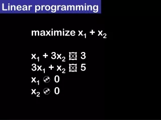
Linear Programming minimize or maximize a linear objective subject to linear equalities and inequalities maximize 3x + 4y subject to 5x + 8y24 x, y 0 A feasible solution satisfies all of the constraints. x = 1, y = 1 is feasible; x = 1, y = 3 is infeasible. An optimal solution is the best feasible solution. The optimal solution is x = 4.8, y = 0.
Terminology • Decision variables: e.g., x and y. • In general, there are quantities you can control to improve your objective which should completely describe the set of decisions to be made. • Constraints:e.g.,5x + 8y24 , x 0 , y 0 • Limitations on the values of the decision variables. • Objective Function. e.g., 3x + 4y • Value measure used to rank alternatives • Seek to maximize or minimize this objective • examples: maximize NPV, minimize cost
Linear Programming (LP) Problem • A mathematical programming problem is one that seeks to maximize an objective function subject to constraints. • If both the objective function and the constraints are linear, the problem is referred to as a linear programming problem. • Linear functions are functions in which each variable appears in a separate term raised to the first power and is multiplied by a constant (which could be 0). • Linear constraints are linear functions that are restricted to be "less than or equal to", "equal to", or "greater than or equal to" a constant.
General Form Of LP Problems MAX (or MIN): c1x1 + c2x2 + … + cnxn Subject to: a11*x1+ a12*x2+…..+ a1n*xn ≤b1a21*x1+ a22*x2+..…+ a2n*xn ≤ b2am1*x1+ am2*x2+..…+ amn*xn ≤ bm, and x1≥ 0, x2 ≥ 0, ....., xn ≥ 0.
Terminology for Solutions • Feasible solution:A solution for which all the constraints are satisfied. It is possible for a problem to have no feasible solutions. Given that there are feasible solutions, the goal of the linear programming is to find which one is the best, as measured by the value of the objective function in the model. • Optimal solution:A feasible solution that has the most favorable value of the objective function. Most favorable value means the largest or the smallest value, depending upon whether the objective is maximization or minimization. • one optimal solution • multiple optimal solutions • no optimal solutions
Solving LP Problems • Graphical Solution Approach - used mainly for 2D problems. • Simplex Method - most common analytic tool.
Steps in Formulating a Linear Programming (LP) Model • Understand the problem. • Identify the decision variables. • State the objective function as a linear combination of the decision variables. • State the constraints: • upper or lower bounds on the decision variables, including non-negativity constraints if applicable. • linear combinations of the decision variables.
A 2-D Maximization Problem Max z = 5x1 + 7x2 s.t. x1< 6 (constraint #1) 2x1 + 3x2< 19 (constraint #2) x1 + x2< 8 (constraint #3) x1, x2> 0 (sign constraint)
Graphical Solution: Constraint #1 x2 8 7 6 5 4 3 2 1 1 2 3 4 5 6 7 8 9 10 x1< 6 (6, 0) x1
Graphical Solution: Constraint #2 x2 8 7 6 5 4 3 2 1 1 2 3 4 5 6 7 8 9 10 (0, 6 1/3) 2x1 + 3x2< 19 (9 1/2, 0) x1
Graphical Solution: Constraint #3 x2 (0, 8) 8 7 6 5 4 3 2 1 1 2 3 4 5 6 7 8 9 10 x1 + x2< 8 (8, 0) x1
Graphical Solution: Combined-Constraint x2 x1 + x2< 8 8 7 6 5 4 3 2 1 1 2 3 4 5 6 7 8 9 10 x1< 6 2x1 + 3x2< 19 x1
Graphical Solution: Optimal Solution x2 8 7 6 5 4 3 2 1 1 2 3 4 5 6 7 8 9 10 5x1 + 7x2 = 46 Optimal Solution x1
Graphical Solution: Five Extreme Points 8 7 6 5 4 3 2 1 1 2 3 4 5 6 7 8 9 10 5 4 Feasible Region 3 1 2 x1
Maximization vs Minimization The position of your optimal point differs, depending upon whether the objective is maximization or minimization. Maximization Minimization Optimum (Max) Isoprofit line Y Y Isocost line Optimum (Min) X X 25
Special Cases • Alternative Optimal Solutions: In the graphical method, if the objective function line is parallel to a boundary constraint in the direction of optimization, there are alternate optimal solutions, with all points on this line segment being optimal. • Infeasibility: A linear program which is over constrained so that no point satisfies all the constraints is said to be infeasible. • Unbounded: Objective function can be maximized infinitely.
Example 2: Unbounded Problem • Solve graphically for the optimal solution (Group Discussion): Max z = 3x1 + 4x2 s.t. x1 + x2> 5 3x1 + x2> 8 x1, x2> 0
Example 2: Unbounded Problem • The feasible region is unbounded and the objective function line can be moved parallel to itself without bound so that z can be increased infinitely. x2 3x1 + x2> 8 8 Max 3x1 + 4x2 5 x1 + x2> 5 x1 2.67 5
Example 3: A Minimization Problem (Group Discussion) Min z = 5x1 + 2x2 s.t. 2x1 + 5x2> 10 4x1 - x2> 12 x1 + x2> 4 x1, x2> 0
Example 3: Graphical Solution Constraints Graphed x2 Feasible Region 5 4 3 2 1 4x1 - x2> 12 x1 + x2> 4 2x1 + 5x2> 10 1 2 3 4 5 6 x1
Example 3: Graphical Solution • Optimal Solution Min z = 5x1 + 2x2 4x1 - x2> 12 x1 + x2> 4 x2 5 4 3 2 1 2x1 + 5x2> 10 Optimal: x1 = 16/5 x2 = 4/5 1 2 3 4 5 6 x1
Graphical Solution to a 2-Variable LP • It can be shown that: • The feasible region for any LP will be a convex set. • The feasible region for any LP has only a finite number of extreme points. • Any LP that has an optimal solution has an extreme point that is optimal.
Fundemental Theorem Of LP (basis of Simplex Method) • If the optimal value of theobjective function in a linearprogramming problem exists, then that value mustoccur at one (or more) of the corner points of the feasible region.
Existence of Solution • (A) If the feasible region for a linear programming problem is bounded, then both the maximum value and the minimum value of the objective function always exist. • (B) If the feasible region is unbounded, and the coefficients of the objective function are positive, then the minimum value of the objective function exists, but the maximum value does not. • (C) If the feasible region is empty (that is, there are no points that satisfy all the constraints), the both the maximum value and the minimum value of the objective function do not exist.
Summary of Graphic Solution • The optimal solution (if one exists) occurs at a “corner point” of the feasible region. • In two dimensions with all inequality constraints, a corner point is a solution at which two (or more) constraints are binding. • There is always an optimal solution that is a corner point solution (if a feasible solution exists). • More than one solution may be optimal in some situations • Graphic solution only works for 2D -> Simplex method.
Gauss-Jordan Algorithm A Key Operation for Numerical LP Algorithm
Gauss-Jordan Method: Principle Gauss-Jordan method is used to solve system of linear equations ( the solution maybe be unique, nonexistent, or infinite ). According to, Ax = b P1P2…P k A x = P1P2…P k b IF P1P2…P k A = I, Then x = P1P2…P k b
Gauss-Jordan: Elementary Row Operations (ero) • Type 1 ero – Matrix A’ is obtained by multiplying any row of A by a nonzero scalar. • Type 2 ero – a row of A (say, row j) is added by another scalar-multiplied row of A (say, row i). • For some j ≠ i, let: row j of A’ = c*(row i of A) + row j of A. • Type 3 ero – Interchange any two rows of A.
Gauss-Jordan: Examples (Group Discussion?) Solve Ax = b where: Step 0 – Write the augmented matrix representation: A|b =
Gauss-Jordan: Column 1 Making a11 the current entry: 1. Multiply row 1 by ½ (type 1 ero). 2. Replace row 2 of A1|b1 by -2*(row1 of A1|b1) + row 2 of A1|b1 (type 2 ero). 3. Replace row 3 of A2|b2 by -1*(row 1 of A2|b2) + row 3 of A2|b2 (type 2 ero). A1|b1 = A2|b2 = A3|b3 =
Making a22 the current entry: 4. Multiply row 2 of A3|b3 by -1/3 (type 1 ero) 5. Replace row 1 of A4|b4 by -1*(row 2 of A4|b4) + row 1 of A4|b4 (type 2 ero). 6. Place row 3 of A5|b5 by 2*(row 2 of A5|b5) + row 3 of A5|b5 (type 2 ero). Gauss-Jordan: Column 2 A4|b4 = A5|b5 = A6|b6 =
Gauss-Jordan: Column 3 • Repeating Step 3 again for the another new entry (a33) and performing an additional three ero’s yields the final augmented array: A9|b9 = Special Cases: After application of the Gauss-Jordan method, linear systems having no solution or infinite number of solutions can be recognized. No solution example: Infinite solutions example:
Gauss-Jordan Method – Basic and Nonbasic variables • Basic variables and solutions to linear equation systems • For any linear system, a variable that appears with a coefficient of 1 in a single equation and a coefficient of 0 in all other equations is called a basic variable. • Any variable that is not a basic variable is called a nonbasic variable. • Let BV be the set of basic variables for A’x=b’ and NBV be the set of nonbasic variables for A’x=b’. The character of the solutions to A’x=b’ ’ (and Ax=b) depends upon which of following cases occur.
Gauss-Jordan: Case 1 -- No Solution Exists Case 1: A’x=b’ has at least one row of the form [0, 0 , …, 0 | c] (c ≠ 0). Then A’x=b’ (and Ax = b) has no solution. In the matrix to the right, row 5 meets this Case 1 criteria. BV = {x1, x2, x3} NBV = {x4} A’|b’ =
Gauss-Jordan: Case 2 -- Only One Solution Exists Case 2: The set of nonbasic variables is empty. Then A’x=b’ will have a unique solution. The matrix to the right has a unique solution. BV = {x1, x2, x3} NBV = {}. A’|b’ =
Gauss-Jordan: Case 3: Infinite Solution Case 3: Suppose Case 1 does not apply and NBV is not empty. Then A’x=b’ (and Ax = b) will have an infinite number of solutions. BV = {x1, x2, and x3} NBV = {x4 and x5}. A’|b’ =
The Gauss-Jordan Method A summary of Gauss-Jordan method is shown to the right. The end result of the Gauss-Jordan method will be one either Case 1, Case 2, or Case 3.
Real LP Problems Real-world LP problems often involve: • Hundreds or thousands of constraints • Large quantities of data • Many products and/or services • Many time periods • Numerous decision alternatives • … and other complications
Standard LP Form An Indispensable Preprocess for Numerical Solution of LP
An LP not in Standard Form maximize3x1 + 2x2 - x3 + x4 x1 + 2x2 + x3 - x4 5; -2x1 - 4x2 + x3 + x4 -1; x1 0,x2 0 Linear Programs in Standard Form We say that a linear program isin standard form if : • 1. Non-negativity constraints for all variables, • 2. All inequality constraints are replaced by equality constraints, and • 3. The right hand side vector,b, is non-negative. not equality not equality x3 may be negative

