Example Project and Numerical Integration
Example Project and Numerical Integration. Computational Neuroscience 03 Lecture 11. Example Project: Investigation into Integrate and fire models. Build a model integrate and fire neuron using. Augmented by the rule that if V reaches V th an AP is fired after which V is reset to V reset

Example Project and Numerical Integration
E N D
Presentation Transcript
Example Project and Numerical Integration Computational Neuroscience 03 Lecture 11
Example Project: Investigation into Integrate and fire models Build a model integrate and fire neuron using Augmented by the rule that if V reaches Vth an AP is fired after which V is reset to Vreset Use EL = -80mV, Vrest = -70mV, Rm= 10MW, tm = 10 ms. Initially set V=Vrest. When the membrane potential reaches Vth = -54mV make the neuron fire a spike and reset the potential to Vreset = -80mV. Show sample voltage traces (with spikes) for a 300ms long current pulse centered in a 500ms long simulation.
Determine the firing rate of the model and compare it with the theoretical prediction:
Investigate the behaviour of this neuron and see how the outputs change if different parameters are modelled. Eg above we see what happens if the current injection is not constant.
Alternatively one could investigate introducing spike rate adaptation by adding a conductance And after a spike is fired Where rmDgsra= 0.06, tsra= 100ms EK=-70mV
Or one can simulate adding an excitatory synaptic conductance with Ie=0 Ps is probability of firing and changes whenever the presynaptic neuron fires using: And after a spike is fired Here use Es = 0 rmgs= 0.5, ts= 10ms Pmax=0.5. Plot V(t) and the synaptic current and trigger synaptic events at times: 50, 150, 190, 300, 320 and 400 Another interesting avenue is to add a calcium-based conductance and see if one can get bursting behaviour Or one can couple 2 IAF neurons etc etc
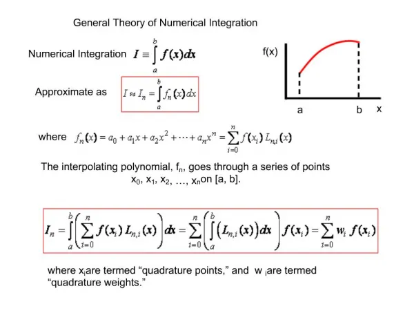
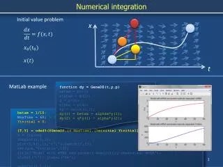
Numerical Integration However whatever scheme one attempts it will be necessary to use some numerical integration (although the equation can be solved for constant Ie). The idea behind numerical integration is very simple and intuitive and can be seen from the following figure: Here we estimate the area under the curve by summing the areas of the trapezium. But what if we are dealing with a differential equation?
Difference Equations Eg consider the IAF equation: The key idea here is to go back to the definition of the differential ie We can then replace the differential (LHS of above) with the finite difference (RHS of above). Alternatively we note that: and iteratively solve: Euler’s method
y(t+h) h dy/dt y(t) t t+h Euler’s method effectively evaluates the function at the future timestep by evaluating the gradient at t and assuming it is constant over the range h Thus the accuracy of y(t+h) is increased (in one sense, see later) by making the increase in time-step h small
y(t+2h) y(t+h) y(t) t t+h t+2h We then iteratively produce the rest of the y-values as illustrated above ie dy/dt evaluated at t+h and h times this value added to y(t+h) to get y(t+2h) etc etc
Can make the reliance of the accuracy of Euler’s method on h explicit by examining the Taylor expansion of y(t) ie: So if we say: y(t+h) = y(t) +h dy/dt +err Then the error term is: Thus for small h the error is determined by the factor h2 ie O(h2) and the method is said to be first order accurate (as we would divide by h to estimate dy/dt) NB note error does also depend on higher order differentials so normally have to assume y is sufficiently smooth
y(t+h) h dy/dt y(t) t t+h However, this procedure is assymetric as we assume dy/dt has a constant value evaluated at beginning of the time interval More symmetric (and accurate) to use an estimate from the middle of the interval ie at h/2 y(t+h) h dy/dt y(t) t t+h t+h/2
y(t+h/2) t t+h/2 t+h However to do this we will need to use the value of y at t+h/2 which we do not yet know Thus we first have to estimate y(t+h/2) using dy/dt evaluated at t and then use this estimate to evaluate dy/dt at t+h/2 as illustrated below: 1 2 Ie if dy/dt= f(y,t): y(t+h/2) = y(t) + h/2 f( y(t), t) (estimate 1 in figure) y(t+h) = y(t) + h f( y(t+h/2), t+h/2) (estimate 2 in figure) This is the 2nd Order Runge-Kutta method
As the name suggests it is 2nd order accurate (method called n’th order if error term is O(hn+1) Why? So comparing this estimate with the Taylor expansion: We see the error is O(h3)
Using a similar procedure but using 4 evaluations of dy/dt we get the commonly used 4th order Runge-Kutta (again dy/dt written as f(y, t) k1 = h f( y(t), t) k2 = h f( y(t)+k1/2, t+h/2) = h f( y(t+h/2), t+h/2) k3 = h f( y(t)+k2/2, t+h/2) k4 = h f( y(t)+k3, t+h) y(t+h) = y(t) + k1/6 + k2/3 + k3/3 + k4/6 + O(h5)
However, note that high order does NOT imply high accuracy: rather it means that the method is more efficient ie quicker to run Generally, for difficult functions (non-smooth) the simpler methods will be more accurate Errors can also arise as a consequence of round-off errors due to computer evaluation Unfortunately, while truncation error reduces as we lower h, round-off errors will increase This results in constraints being placed on step-sizes used so that algorithm remains stable and round-off errors do not swamp the solution
Note that one can get an estimate of the gradient from an advanced timestep (forward differencing) or from a previous timestep (backward difference) Using forward differences (or mix of forwards and backwards) is a lot more computationally intensive as we then have to solve a set of simultaneous equations (though system is usually tridiagonal), but often need to do so as these schemes (implicit) are much more stable
EG: IAF equation Back to the IAF equation: Becomes: Where timestep is 1 ms (as long as it doesn’t vary too quickly).
If there are gating variables for conductances etc they can be integrated in the same way eg These should be updated at different times to the voltage ie if V is computed at times 0, t, 2t, 3t etc, then z would be updated at times t/2, 3t/2, 5t/2 etc If calcium based conductances are included, they should be updated simultaneously with V Also, remember that if you can analytically integrate an equation you should eg