Download
1 / 31
310 likes | 420 Vues
This tutorial in MSC Patran 2005 r2 covers modeling, analyzing a cantilevered beam with a mid-span support, determining max/min deformation and stress, creating a comprehensive report file. Follow step-by-step instructions for creating the model database, setting up analysis, creating points, curves, mesh, and applying boundary conditions. Experience Level: Lower MD. Estimated Time: ~30 min.

E N D
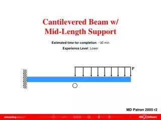
P Cantilevered Beam w/ Mid-Length Support Estimated time for completion: ~30 min Experience Level: Lower MD Patran 2005 r2
Topics Covered • Using a total load to apply a uniform distributed load over an given length • Creating a boundary condition that does not go into effect until a certain deformation • Using 1-D beam element • Orientation of beam • Geometric properties of beam (cross-sectional area) • Showing true deformation results (to scale) • Creating results report of relevant information
Problem Description 20 ft P =1,000 lbf y x h = 7 in 0.5 in 20 ft 20 ft • The solid rectangular beam is cantilevered in the left side • Roller support at the mid-span • Note: at initial condition the roller support is not in contact with beam • Has uniform distributed load in the right end of the beam • Weight of the beam is to be ignored Elasticity Modulus = 30x106 psi Poisson’s Ratio = 0.3 width = 3.5 in Note: Diagram not to scale.
Goal • Model the Cantilevered beam with mid-length support and analyze the structure. Determine the maximum and minimum deformation and combined stresses. • Is the downward force large enough to cause a deflection that will allow the beam to contact with the mid-span roller? • Create a report file with all the relevant information for such analysis.
Expected Results Bar Stress: Combined Stress Maximum Stress 4.20x10³ psi @ node 2 Minimum Stress 3.49x10⁻⁵ psi @ node 4 Displacement: Translational Maximum Displacement 2.40 in @ node 4 Minimum Displacement 0 in @ node 1
Starting MSC.Patran from Windows To start MSC.Patran from a windows computer you will have to: • Click on start menu • Roll mouse over All Programs • Roll mouse over MSC.Software • Roll mouse over MSC.Patran 2005 r2 • Click on MSC.Patran 2005 r2
Creating a New Database • Click File menu / Select New. • In the File name text field enter beam_midsupport. • Click OK. Note: MSC.Patran defaults the working folder to C:/windows/temp. Make sure the folder content is deleted before starting a new database.
Database Settings for the Model • Select Tolerance radio button: Based on Model. • Enter in the Approximate Maximum Model Dimension textfield: 480Note: This is the largest dimension of your model to be analyzed which allocates enough space to create your geometry • Select Analysis Code to be MSC.Nastran from the drop down menu • Select Analysis Type to be Structural from the drop down menu since the model that you are about to analyze is a truss structural problem. • Click OK. a b c d e Remember: MSC.Patran does not handle units of measurement, so it is essential to remember to use one consistent system of measurement. In this example, SI units are used with the following measuring units: Input Output Length meters Force Newtons Elastic Modulus Pa Mass kg Displacement meters Force Newtons Stress Pa
Creating Points Using XYZ Method f a b • Click on Geometry icon. • Select Create / Point / XYZ from the drop down menus. • Uncheck Auto Execute. • In the Point Coordinate List text field enter [0 0 0]. • Click on Apply button. • Click on Label Control. • Click on Point. • Repeat steps (d) through (e) with the mid-span point [240 0 0] and right end point [480 0 0] c d e g
Creating Curves by Connecting Two Points • Select Create / Curve / Point from the drop down menus. • In the Option drop down menu select 2 Point. • Click in the Starting Point List text field and click on the left most point(Point 1) on the viewport window. • Click on the Ending Point List text field and click on the middle point (Point 2) of the viewport window. • Click Apply button. • Repeat previous step but connecting the middle point (Point 2) with the point furthest to the right (Point 3). a b c d e
Creating Mesh Seed from the Curves a • Click on Element icon. • Select Create / Mesh Seed / Uniform from the drop down menu. • Select Number of Elements radio button. • In the Number text field enter 1. • Make sure Auto Execute checkbox is off. • Click on the Curve List text field. To select both curves, click and drag a square over the beam structure. • Click on Apply button. b c d e f g
Creating Mesh • Select Create / Mesh / Curve from the drop down menus. • From the Topology drop down menu select Bar2. • In the Curve List text field, select both curves again by dragging a box around the beam structure. • The Global Edge checkbox off. • Click Apply Button. a b c d e
Equivalencing Nodes with Tolerance Cube • Select Equivalence / All / Tolerance Cube from the drop down menus. • In the Equivalencing Tolerance textbox enter 0.001. • Click on Apply button. • Note in the History Window that 1 node have been eliminated. a b c d
Creating Boundary Condition for Cantilever a • Click on Load/BCs icon. • Select Create / Displacement / Nodal from the drop down menus. • Enter New Set Name to be cantilevered. • Click on Input Data… button. • In the Translation textbox enter <0 0 0> • In the Rotation textbook enter <0 0 0> • Click Ok button. • Click on Application Region button. • Under Geometry Filter select Geometry radio button. • In the Select Geometry Entities textbox click on Point 1 (left point). • The Selection window will appear which Point 1 should be clicked. • Click Add button • Click OK button. • Click Apply button. b i e f j l g m c d h k n Note: In the viewport, point 1 is constrained in 1,2,3,4,5,6 directions
Creating Boundary Condition for Mid-Length Support h • Select Create / Displacement / Nodal from the drop down menus. • Enter New Set Name to be center_roller. • Click on Input Data… button. • In the Translation textbox enter < , -0.5, > • In the Rotation textbook enter < > • Click Ok button. • Click on Application Region button. • Under Geometry Filter select Geometry radio button. • In the Select Geometry Entities textbox click on Point 2 (center point). • The Selection window will appear which Point 2 should be clicked. • Click Add button • Click OK button. • Click Apply button. a d e i k l f b c g m j
Creating Distributed Load • Select Create / Total Load / Element Uniform from the drop down menus. • In the New Set Name textbox enter total_load. • Select Target Element Type to be 1D from the drop down menu. • Click on Input Data… button. • In the Load text-field enter <0 -1000 0>. • Click on OK button. • Click on Select Application region… button. • In the Geometry Filter, select Geometry radio button. • In the Select Geometry Entities text-field click on the right curve (the curve starting from the mid-support to the right free end) • Click Add button. • Click OK button. • Click Apply button. a h e i j k b f c d g l
Summarizing Load / Boundary Conditions • In the cantilevered side, no translational nor rotational displacement is allowed which means that all 6 degrees of freedom are constrained. Thus, the numbers 1,2,3,4,5,6 are shown to be constrained. • At the mid-length, a constrained in the y-direction is applied. But such constrain does not go into action until it has moved 5 inches down, thus, the -5. • There is a total uniform distributed load of 1,000 lbf downwards. b c a
Creating Material Properties a • Click on Material icon. • Select Create / Isotropic / Manual Input from the drop down menus. • In the MaterialName text field enter steel. • Click on InputProperties… button. • From the Constitutive Model select Linear Elastic from the drop down menus. • In the Elastic Modulus text field enter 30e6. • For the Poisson Ratio enter 0.3. • Click OK button. • Click Apply button.
Applying Material Properties to Beam a b • Click on Properties icon. • Select Create / 1D / Beam from the drop down menus. • In Property Set Name text field enter beam_prop. • Click on Input Properties… button. • Click on Mat Prop Name button. • Select steel by clicking it. • Click on Create Section Beam Library. e f g c d
Applying Beam Properties a • Select Create / StandardShape / NastranStandard from the drop down menus. • In the New Section Name text field enter beam_1. • Click on the left or right arrows to toggle through the options until the solid rectangle appear. • Click on the solid rectangle. • In the Width (W) text field enter 3.5. • In the Height (H) text field enter 4. • Click on Calculate / Display button. • In the Section Display Window make sure that the moment of inertia I = 100 in4. • Click on OK button h e f b d c g i
zel yel xel Let’s step aside from the tutorial procedures so the beam orientation can be better explained: The orientation vector of the beam (N) is defined to be the normal vector to the xel -yel plane. To orient this beam in space for the model, the vector N will be used to orient the beam with the Global coordinate system. A few examples of how the bar orientation vector changes in position. N Global Coordinate Sys. Z <1 0 0> Y <-1 0 0> X <0.2 0 1>
Applying Beam Properties f g • Since the Orientation of the beam does not change, in the Bar Orientation text field enter <0 1 0> • Click OK button. • In the Select Members text box, click on the text field and select both curves. • Click Add button. • Click Apply button. • To display the beam geometry in the viewport window you will have to go follow these steps:Display Menu Load/BS/Elem. Props… Under beam display select 3D FullSpan+Offset from the drop down menu and then click on Apply Button • Optional: select one of the 3 rendering icons to enhance the view of your structure. a b c d e
Analyzing Model a • Click on Analysis icon. • Select Analyze / Entire Model / Full Run from the drop down menus. • Click on Translation Parameters… button. • Make sure the checkbox for XDB and Printer is On. Use default setting for the other options. • Click OK button. • Click on Solution Type… button. • Make sure the Linear Static radio button is selected. • Click OK button. • Click Apply button. d b g c f h i e
Loading the Results File Output from Nastran • Select Access Results / Attach XDB / Results Entities from the drop down menus. • Click on Select Results File… button. • Click on beam_midsupport.xdb • Click OK button. • Click Apply button. a c d b e
Displaying Result Plot: Bar Stresses, Maximum Combined a • Click on Results icon. • Select Create / Quick Plot from the drop down menus. • Under Select Results Cases click on SC1: DEFAULT, A1: Static Subcase. • Under Select Fringe Result click on Bar Stresses, Maximum Combined. • Under Select Deformation Result select Displacements, Translational. • Click Apply button. b c d e f
Displaying Result Plot: True Displacement Plot When Creating a deformation plot, usually the deformation is exaggerated for illustration purposes. But it is useful to sometimes see the true deformation that the model is undergoing to have an accurate feel for the model. • Select Create / Quick Plot from the drop down menus. • Under Select Results Cases select Default, A1: Static Subcase • Under Select Fringe Result select Displacement, Translational • Select under the Quantity drop down menu Magnitude • Under Select Deformation Result, select Displacement, Translational • Click on Displacement icon • Under Scale Interpretation select the True Scale radio button. • In the Scale Factor text box enter 1.0 • Click Apply button. a f b g h c d e i
Creating Results Report • Select Create / Report / Append File from the drop down menus. • Under Select Result Case select Default, A1: Static Subcase • Under Select Report Result select Bar Stresses, Maximum Combined. • From the Select Quantities click on Scalar Value • Click Apply Button. • A new file called Patran.rpt will be created in the default directory. Double click to open such file. (If windows requests which program to open it with, select NotePad) a b f c d e Note: If more information is needed to in the report file, go ahead and select the information using similar method as above and make sure the append method is selected. This will just keep on writing the results after the last line on that report file.
Summary of Results of FEA Bar Stress: Combined Stress Maximum Stress 4.20x10³ psi @ node 2 Minimum Stress 3.49x10⁻⁵ psi @ node 4 Displacement: Translational Maximum Displacement 2.40 in @ node 4 Minimum Displacement 0 in @ node 1
Important Skills Acquired • Using a total load to apply a uniform distributed load over an given length • Creating a boundary condition that does not go into effect until a certain deformation • Using 1-D beam element • Orientation of beam • Geometric properties of beam (cross-sectional area) • Showing true deformation results (to scale) • Creating results report of relevant information
Further Analysis (Optional) • Run the analysis again changing the mid-length boundary condition to be initially touching the beam meaning that no displacement will be allowed in the y-direction. Compare the resulting stresses and deformation with the previous conditions. • The beam used in this example was a solid rectangular beam. To optimize the design and cut costs (by reducing material) use a different beam geometry/dimension to optimize the design. (The stresses and deflection should be either equal or less than the actual obtained in this tutorial)
Best Practices • When using 1-D beam elements it is essential to know the geometric measurement for the cross sectional area and beam orientation. • The orientation of the beam is crucial for the proper analysis, a wrongly orientated beam can introduce immeasurable error to the results. (ie, loading an I-beam in the wrong direction)