Statapult Exercise
Statapult Exercise. Launch #1 Using what you are given, baseline the process for shooting the statapult . Remember: Customer desires a rapid-fire, precise, and accurate launcher that can launch projectiles over mountain ranges. Group Activity.

Statapult Exercise
E N D
Presentation Transcript
Launch #1 Using what you are given, baseline the process for shooting the statapult. Remember: Customer desires a rapid-fire, precise, and accurate launcher that can launch projectiles over mountain ranges. Group Activity
Every shot will be launched from a pull back angle of 177/65 degrees. Each person on the team will perform an equitable number of launches (or as close as possible). "Launching” means pulling back and releasing. Time between each shot cannot exceed 15 seconds. Record the distances on the table to the left. Record the longest distance (Max) and the shortest distance (Min) and compute Range = Max - Min. Statapult Instructions Launch #1 Objective: To fire the statapult and record the distance for each of the launches. The measured distance will be from the back of the launcher to the point where the ball first lands. Record the distances in the order in which they were obtained. Range = ______________
StatapultLaunch #1 See graphing.pdf VI-19
Sigma Values • Short term data is considered free of assignable causes • One shift, one operator • Long term data is considered to contain both assignable and common caused variation • Multiple shifts, multiple operators • Processestend to exhibit more variation in the long term than the short VI-8
Levels of Maps Maps can be created for many different levels of the process. Just like highway maps… You can use a map of the USA… or if you need more detail, a map of the state... or if you need more detail, a map of the city. Mapping works much the same way. Depending on the detail you need, create the map at that level. If you need more detail, then create a more detailed map of the sub-process. High Level Detail VI-27
High Level Process Map • Process Flow Diagram • Used to identify the steps in a process • Good for process documentation and knowledge gathering • May be used in definition, detail design, analysis and control portions of a project Visually sets the process steps in order VI-27
Swim Lane (Functional or Deployment Maps) • To provide a graphical representation of the process with regards to • the people involved, • their responsibilities, • functional interfaces and dependencies, • as well as process steps over time where necessary. • Critical tool for transactional processes and when mapping information flow for industrial processes • Segregates steps by who does them or where they are done • Makes handoffs visible A Swim Lane is a process flow diagram with resource responsibilities VI-27
Functional or Deployment Flow Diagram Process Steps Business Unit Review & approve Define needs Prepare paperwork Receive & use Configure & install Review & approve standard I.T. Issue payment Finance Review & approve Top Mgt/ Corporate Review & approve Resources Responsible for Process Steps Acquire equipment Sourcing Supplier Supplier Graphical summary or roles & responsibilities for a process VI-27
Process Flow Chart Objective: Develop a process flow diagram that explains the current process of how to launch a ball. VI-27
SIPOC Supplier Customer Process Input Output SIPOC is a process scoping tool that provides a high level definition of a process –SIPOC should be used on all Six Sigma projects VI-4
Boundary 2 When does the Process start? 2 When does the process end? Boundary SIPOC – The Process Steps 6 What Inputs are required to enable this process to occur? 3 What are the outputs from the process? 4 Who is the customer of each output? 1 What is the process? 7 Who is the supplier of each input? 8 What does the process expect from each input? 5 What does each customer expect from each output? VI-4
Group Exercise - SIPOC PROCESS INPUTS OUTPUTS VI-4
Relationship Matrix • Create a relationship matrix for the previous SIPOC *Input/Output relationships can be rated as: Strong: 9 Moderate: 3 Weak: 1 Nonexistent: Blank or 0 V-28
Basic Structure – C&E Diagram(Fishbone) C = Control Factor (controllable) N = Noise factor (out of our control) X = Experimental variable Inputs (X’s) Output (Y) Main Category People Measurements Materials C Level 1 Cause C N N Level 2 Cause Project Y N C X C X Environment Methods Machines By identifying the correct inputs, you can achieve optimal results in the shortest time. VIII-133
Cause & Effect C/N/X’s C =those variables which must be held constant and require standard operating procedures to insure consistency. Consider the following examples: the method used to enter information on a billing form, the method used to load material in a milling or drilling process, the autoclave temperature setting. N = those variables which are noise or uncontrolled variables and cannot be cheaply or easily held constant. Examples are room temperature or humidity. X = those variables considered to be key process (or experimental) variables to be tested in order to determine what effect each has on the outputs and what their optimal settings should be to achieve customer-desired performance. VIII-133
MANPOWER METHOD MACHINE MOTHER MEASUREMENT MATERIAL NATURE Cause and Effect Diagram Objective: Develop a C&E diagram that explains the variability of the launching process. Label as C/N/X. VIII-133
FMEA • In groups • Conduct a process FMEA for “shooting the statapult” • Generate Risk Priority Numbers and develop controls that will minimize risk VII-116
SOP Objective: Develop a SOP that accurately defines each controlled step of the improved launching process. VI-30
Every shot will be launched from a pull back angle of 177/65 degrees. Each person on the team will perform an equitable number of launches (or as close as possible). "Launching” means pulling back and releasing. Time between each shot cannot exceed 15 seconds. Record the distances on the table to the left. Record the longest distance (Max) and the shortest distance (Min) and compute Range = Max - Min. Statapult Instructions Launch #2 Objective: To fire the statapult and record the distance for each of the launches. The measured distance will be from the back of the launcher to the point where the ball first lands. Record the distances in the order in which they were obtained. Range = ______________
StatapultLaunch #2 See graphing.pdf VI-19
Concentration Chart http://www.qualitytrainingportal.com/resources/problem_solving/problem-solving_tools-concentration_diagrams.htm www.duetsblog.com/uploads/image/AT&T.jpg VI-46
Population vs. Sample Population • Data is collected using samples because the entire population may not be known or it may be too costly to measure. • Population is every possible item • Sample is a subset of the population Sample VII-2
Calculating Standard Deviation • Step #1 Add the data points and divide by the number of data point to determine the mean (average) • Step #2 Subtract the mean from each individual data point and square the result (data point – Mean)2 • Step #3 Add together all the squared data points • Step #4 Divide the total of the squared data points by n-1 if a sample, or n if a population (n= number of data points) • Step #5 Calculate the square root of the sum of step #4.The result is the standard deviation for the process. VI-8
Launch #1 VI-8
Launch #2 VI-8
Graphical View of Variation and Six Sigma Performance Each unit of measure is a numerical value on a continuous scale Variation common and special causes Pieces vary from each other Size Size Size Size But they form a pattern that, if stable, is called a normal distribution Normal Distribution Histogram or Frequency Distribution VII-31
Normal Distribution There are three terms used to describe distributions 1. Shape Bell 2. Spread Standard Deviation • 3. Location • Mean VII-31
Y=f(x) Scatter Diagram Example: Distance Angle VII-16
Histogram examples VII-20
Histogram examples VII-20
Computing Cost Of Poor Quality • Instructions • Refer to Launch #1 and #2 and convert the run charts shown on these pages to histograms, using 4-inch intervals as the class width. • The student may then choose the 12-inch range (3 consecutive 4-inch intervals) centered around the average to be the specification range. • Draw those spec limits on the histogram and complete the following table: Launch #1 Launch #2 III-26
Dev. from Heights Avgerage. Total Xbar » Sigma!! (average) Calculate our statistics Let’s practice Find: Mean Median Mode Range Sigma -population -sample 5’ = 60” 6’ = 72”
Xbar = Step 2 Create a Histogram - (Use 2" Scale increments) Sigma Area % Height Span Realistic? (Y/N) +/- 1 Sigma +/- 2 Sigma +/- 3 Sigma +/- 6 Sigma Plot height data and use the statistics Step 3 Add Sigma Limits Step 4 Analyze

![[Exercise Name] Functional Exercise](https://cdn0.slideserve.com/621913/exercise-name-functional-exercise-dt.jpg)

![[Exercise Name] Functional Exercise](https://cdn1.slideserve.com/1717560/exercise-name-functional-exercise-dt.jpg)


![[Exercise Name] Functional Exercise](https://cdn3.slideserve.com/6680259/exercise-name-functional-exercise-dt.jpg)
![[Exercise Name] Tabletop Exercise](https://cdn4.slideserve.com/9191716/exercise-name-tabletop-exercise-dt.jpg)