Eddy Current Maths
Eddy Current Maths

Eddy Current Maths
E N D
Presentation Transcript
Electromagnetic Testing - Eddy Current Mathematics 2014-December My ASNT Level III Pre-Exam Preparatory Self Study Notes 外围学习中 Charlie Chong/ Fion Zhang
Fion Zhang at Shanghai 2014/November http://meilishouxihu.blog.163.com/ Shanghai 上海 Charlie Chong/ Fion Zhang
Impedance Phasol Diagrams Charlie Chong/ Fion Zhang
Impedance Phasol Diagrams Charlie Chong/ Fion Zhang
Greek letter Charlie Chong/ Fion Zhang
Eddy Current Inspection Formula Charlie Chong/ Fion Zhang https://www.nde-ed.org/GeneralResources/Formula/ECFormula/ECFormula.htm
Charlie Chong/ Fion Zhang https://www.nde-ed.org/GeneralResources/Formula/ECFormula/ECFormula.htm
Charlie Chong/ Fion Zhang https://www.nde-ed.org/GeneralResources/Formula/ECFormula/ECFormula.htm
Charlie Chong/ Fion Zhang https://www.nde-ed.org/GeneralResources/Formula/ECFormula/ECFormula.htm
Charlie Chong/ Fion Zhang https://www.nde-ed.org/GeneralResources/Formula/ECFormula/ECFormula.htm
Units Charlie Chong/ Fion Zhang
Ohms Law: According to Ohms Law, the voltage is the product of current and resistance. V = I x R Where V = Voltage in volts, I = Current in Amps and R = Resistance in Ohms Inductance of a solenoid is given by: L=μoN2A/l https://en.wikipedia.org/wiki/Inductance Charlie Chong/ Fion Zhang
Phase Angle and Impedance Phase angle is expressed as follows: tan Φ = XL/R Where: Φ = Phase Angle in degrees, XL= Inductive Reactance in ohms and R = Resistance in ohms. Impedance is defined as follows: Where Z = Impedance in ohms, R = Resistance in ohms and XL= Reactance in ohms. Charlie Chong/ Fion Zhang
Magnetic Permeability and Relative Magnetic Permeability Magnetic permeability is the ratio between magnetic flux density and magnetizing force. μ =B/H Where μ = Magnetic Permeability in Henries per meter (mu), B = Magnetic Flux Density in Tesla, H = Magnetizing Force in Amps/meter. Relative magnetic permeability is expressed as follows: μr= μ / μo Where μr = Relative magnetic permeability (mu) and μo= Magnetic permeability of free space (Henries per meter = 1.257 * 10-6). μr= 1 for non- ferrous materials. Charlie Chong/ Fion Zhang
Conductivity and Resistivity Conductivity and resistivity is related as follows: σ =1/ ρ Where σ = Conductivity (sigma) and ρ =Resistivity (rho). Conductivity can be quantified in Siemens per m (S/m) or in Aerospace NDT in % lACS (International Annealed Copper Standard). One Siemen is the inverse of an ohm. Another common unit used for conductivity measurement is Siemen per cm (S/cm). Charlie Chong/ Fion Zhang
Electrical Conductivity and Resistivity Resistance can be defined as follows: R = l /(Aσ) or R = ρl/A Where: R = the resistance of a uniform cross section conductor in ohms (Ω), l = the length of the conductor in the same linear units as the conductivity or resistivity is quantified, A=Cross Sectional area, σ = conductivity in S/m and ρ = Resistivity in Ω m. Charlie Chong/ Fion Zhang
In eddy current testing, instead of describing conductivity in absolute terms, an arbitrary unit has been widely adopted. Because the relative conductivities of metals and alloys vary over a wide range, a conductivity benchmark has been widely used. In 1913, the International Electrochemical Commission established that a specified grade of high purity copper, fully annealed - measuring 1 m long, having a uniform section of 1 mm2 and having a resistance of 17.241 mΩ at 20°C (1.7241x10⁻⁸ohm-meter at 20°C) - would be arbitrarily considered 100 percent conductive. The symbol for conductivity is σ and the unit is Siemens per meter. Conductivity is also often expressed as a percentage of the International Annealed Copper Standard (IACS). Charlie Chong/ Fion Zhang
Conductivity & Resistivity Temperature Coefficient of Resistance** Tensile Strength (lbs./sq. in.) Relative Conductivity* Metal Aluminum (2S; pure) 59 0.0039 30,000 Aluminum (alloys): · Soft-annealed · Heat-treated 45-50 30-45 — — — — Brass 28 0.002-0.007 70,000 Cadmium 19 0.0038 — Chromium 55 — — Cobalt 16.3 0.0033 — Constantin 3.24 0.00001 120,000 Copper: Hard drawn · Annealed 89.5 100 0.00382 0.00393 60,000 30,000 Gold 65 0.0034 20,000 Charlie Chong/ Fion Zhang http://www.wisetool.com/designation/cond.htm
Conductivity & Resistivity Iron: · Pure · Cast · Wrought 17.7 2-12 11.4 0.005 — — — — — Lead 7 0.0039 3,000 Magnesium — 0.004 33,000 Manganin 3.7 0.00001 150,000 Mercury 1.66 0.00089 0 Molybdenum 33.2 0.004 — Monel 4 0.002 160,000 Nichrome 1.45 0.0004 150,000 Nickel 12-16 0.006 120,000 Charlie Chong/ Fion Zhang
Conductivity & Resistivity Nickel silver (18%) 5.3 0.00014 150,000 Phosphor bronze 36 0.0018 25,000 Platinum 15 0.003 55,000 Silver 106 0.0038 42,000 Steel 3-15 0.004-0.005 42,000-230,000 Tin 13 0.0042 4,000 Titanium 5 — 50,000 Titanium, 6A14V 5 — 130,000 Tungsten 28.9 0.0045 500,000 Zinc 28.2 0.0037 10,000 Charlie Chong/ Fion Zhang
FIGURE 13. Normalized impedance diagram for long coil encircling solid cylindrical non-ferromagnetic bar and for thin wall tube. Coil fill factor = 1.0. Legend k = √(ωμσ) = electromagnetic wave propagation constant for conducting material r = radius of conducting cylinder (m) μ = magnetic permeability of bar (4 πx10–7 H·m-1if bar is nonmagnetic) σ= electrical conductivity of bar (S·m-1) ω = angular frequency = 2πf where f = frequency (Hz) √(ω L0G) = equivalent of √(ωμσ) for simplified electrical circuits, where G = conductance (S) and L0= inductance in air (H) Charlie Chong/ Fion Zhang
Legend k = √(ωμσ) = electromagnetic wave propagation constant for conducting material r = radius of conducting cylinder (m) μ = magnetic permeability of bar (4 π x10–7H·m-1if bar is nonmagnetic) σ = electrical conductivity of bar (S·m-1) ω = angular frequency = 2 π f where f = frequency (Hz) √(ω L0G) = equivalent of √(ωμσ) for simplified electrical circuits, where G = conductance (S) and L0= inductance in air (H) Keywords: ? δ = √(2/ωμσ) = 1/√(ωμσ) = 1/k = 1/(π f μσ)½ For √(ω L0G) = √(ωμσ) , L0G = μσ Charlie Chong/ Fion Zhang
The magnetic permeability μ is the ratio of flux density B to magnetic field intensity H: μ = B∙H-1 where B = magnetic flux density (tesla) and H = magnetizing force or magnetic field intensity (A·m–1). In free space, magnetic permeability μ0= 4 π × 10–7H·m–1. Charlie Chong/ Fion Zhang
Magnetic permeability of free space: μ0= 4 π × 10–7H·m–1 Charlie Chong/ Fion Zhang
Magnetic Permeability Magnetic Flux: Magnetic flux is the number of magnetic field lines passing through a surface placed in a magnetic field. ϴ We show magnetic flux with the Greek letter; Ф. We find it with following formula; Ф =B∙A ∙ cos ϴ Where Ф is the magnetic flux and unit of Ф is Weber (Wb) B is the magnetic field and unit of B is Tesla A is the area of the surface and unit of A is m2 Following pictures show the two different angle situation of magnetic flux. Charlie Chong/ Fion Zhang http://www.physicstutorials.org/home/magnetism/magnetic-flux-and-magnetic-permeability
In (a), magnetic field lines are perpendicular to the surface, thus, since angle between normal of the surface and magnetic field lines 0° and cos 0° =1 equation of magnetic flux becomes; Ф =B ∙ A In (b), since the angle between the normal of the system and magnetic field lines is 90° and cos 90° = 0 equation of magnetic flux become; Ф =B ∙ A ∙ cos 90° = B ∙ A ∙ 0 = 0 (a) (b) Charlie Chong/ Fion Zhang http://www.physicstutorials.org/home/magnetism/magnetic-flux-and-magnetic-permeability
Magnetic Permeability - In previous units we have talked about heat conductivity and electric conductivity of matters. In this unit we learn magnetic permeability that is the quantity of ability to conduct magnetic flux. We show it with µ. Magnetic permeability is the distinguishing property of the matter, every matter has specific µ. Picture given below shows the behavior of magnetic field lines in vacuum and in two different matters having different µ. Charlie Chong/ Fion Zhang http://www.physicstutorials.org/home/magnetism/magnetic-flux-and-magnetic-permeability
Magnetic permeability of the vacuum is denoted by; µoand has value; µo = 4 π.10-7 Wb/Amps.m We find the permeability of the matter by following formula; µ= B / H Where; H is the magnetic field strength and B is the flux density Relative permeability is the ratio of a specific medium permeability to the permeability of vacuum. µr=µ/µo Charlie Chong/ Fion Zhang http://www.physicstutorials.org/home/magnetism/magnetic-flux-and-magnetic-permeability
Diamagnetic matters: If the relative permeability f the matter is a little bit lower than 1 then we say these matters are diamagnetic. Paramagnetic matters: If the relative permeability of the matter is a little bit higher than 1 then we say these matters are paramagnetic. Ferromagnetic matters: If the relative permeability of the matter is higher than 1 with respect to paramagnetic matters then we say these matters are ferromagnetic matters. Charlie Chong/ Fion Zhang http://www.physicstutorials.org/home/magnetism/magnetic-flux-and-magnetic-permeability
Magnetic Permeability Charlie Chong/ Fion Zhang http://www.physicstutorials.org/home/magnetism/magnetic-flux-and-magnetic-permeability
Standard Depth Charlie Chong/ Fion Zhang
Standard Depth of Penetration Standard depth of penetration is given as follows: Where δ = standard depth of penetration in m; f = frequency (Hz); μ = Magnetic Permeability (Henries per meter); and σ = conductivity in S/m. The influence of frequency and conductivity on standard depth of penetration is illustrated in Figure 1. Charlie Chong/ Fion Zhang
Figure 1. Influence of frequency and conductivity on standard depth of penetration. Charlie Chong/ Fion Zhang
Current Density Change with Depth The change in current density with depth is expressed as follows: Jx= Joe–x/δ Where Jx= Current Density at distance x below the surface (amps/m2); J0 = Current Density at the surface (amps/m2); e = the base of the natural logarithm (Euler's number) = 2.71828; x = Distance below the surface; and δ = standard depth of penetration in meters. Charlie Chong/ Fion Zhang
Depth of Penetration and Probe Size Smith et al have introduced the idea of spatial frequency. Where D = the effective diameter of the probe field in meters, limiting the depth of penetration to D/4. The probe effective diameter is considered to be infinite in the usual equation. Charlie Chong/ Fion Zhang
Depth of Penetration & Current Density Charlie Chong/ Fion Zhang http://www.suragus.com/en/company/eddy-current-testing-technology
Standard Depth Calculation Where: μ = μ0x μr Charlie Chong/ Fion Zhang
The applet below illustrates how eddy current density changes in a semi- infinite conductor. The applet can be used to calculate the standard depth of penetration. The equation for this calculation is: Where: δ = Standard Depth of Penetration (mm) π = 3.14 f = Test Frequency (Hz) μ = Magnetic Permeability (H/mm) σ = Electrical Conductivity (% IACS) Charlie Chong/ Fion Zhang
Defect Detection / Electrical conductivity measurement (1/e)3or 5% of surface density at material interface 1/e or 37% of surface density at target Defect Detection Electrical conductivity measurement Charlie Chong/ Fion Zhang
The skin depth equation is strictly true only for infinitely thick material and planar magnetic fields. Using the standard depth δ , calculated from the above equation makes it a material/test parameter rather than a true measure of penetration. (1/e) (1/e)2 (1/e)3 FIG. 4.1. Eddy current distribution with depth in a thick plate and resultant phase lag. Charlie Chong/ Fion Zhang
Sensitivity to defects depends on eddy current density at defect location. Although eddy currents penetrate deeper than one standard depth (δ) of penetration they decrease rapidly with depth. At two standard depths of penetration (2δ ), eddy current density has decreased to (1/ e)2or 13.5% of the surface density. At three depths (3δ), the eddy current density is down to only (1/ e)3or 5% of the surface density. However, one should keep in mind these values only apply to thick sample (thickness, t > 5r ) and planar magnetic excitation fields. Planar field conditions require large diameter probes (diameter > 10t) in plate testing or long coils (length > 5t) in tube testing. Real test coils will rarely meet these requirements since they would possess low defect sensitivity. For thin plate or tube samples, current density drops off less than calculated from Eq. (4.1). For solid cylinders the overriding factor is a decrease to zero at the centre resulting from geometry effects. Charlie Chong/ Fion Zhang
One should also note that the magnetic flux is attenuated across the sample, but not completely. Although the currents are restricted to flow within specimen boundaries, the magnetic field extends into the air space beyond. This allows the inspection of multi-layer components separated by an air space. The sensitivity to a subsurface defect depends on the eddy current density at that depth, it is therefore important to know the effective depth of penetration. The effective depth of penetration is arbitrarily defined as the depth at which eddy current density decreases to 5% of the surface density. For large probes and thick samples, this depth is about three standard depths of penetration. Unfortunately, for most components and practical probe sizes, this depth will be less than 3δ , the eddy currents being attenuated more than predicted by the skin depth equation. Keywords: For large probes and thick samples, this depth is about three standard depths of penetration. Unfortunately, for most components and practical probe sizes, this depth will be less than 3δ. Charlie Chong/ Fion Zhang
Standard Depth of Penetration Versus Frequency Chart Charlie Chong/ Fion Zhang https://www.nde-ed.org/GeneralResources/Formula/ECFormula/DepthFreqChart/ECDepth.html
Magnetic Field & Size of Coil Typically, the magnetic field β in the axial direction is relatively strong only for a distance of approximately one tenth of the coil diameter, and drops rapidly to only approximately one tenth of the field strength near the coil at a distance of one coil diameter. D=Coil diameter 0.1D β0 D 0.1β0 Charlie Chong/ Fion Zhang
Flaw Detection Depth To penetrate deeply, therefore, large coil diameters are required. However as the coil diameter increases, the sensitivity to small flaws, whether surface or subsurface, decreases. For this reason, eddy current flaw detection is generally limited to depths most commonly of up to approximately 5 mm only, occasionally up to 10 mm. For materials or components with greater cross-sections, eddy current testing is usually used only for the detection of surface flaws and assessing material properties, and radiography or ultrasonic testing is used to detect flaws which lie below the surface, although eddy current testing can be used to detect flaws near the surface. However, a very common application of eddy current testing is for the detection of flaws in thin material and, for multilayer structures, of flaws in a subsurface layer. Charlie Chong/ Fion Zhang
Phase Lag Charlie Chong/ Fion Zhang