Advanced Eddy Current NDE Techniques & Applications
Explore the principles, instrumentation, and applications of Eddy Current Non-Destructive Evaluation. Learn about inspection techniques, including single and multiple frequencies, as well as specialized instrumentation for accurate results. Discover typical applications such as conductivity and permeability measurements, metal and coating thickness assessments, and flaw detection in various materials.

Advanced Eddy Current NDE Techniques & Applications
E N D
Presentation Transcript
3 Eddy Current NDE 3.1 Inspection Techniques 3.2 Instrumentation 3.3 Typical Applications 3.4 Special Example
voltmeter voltmeter voltmeter oscillator oscillator oscillator ~ ~ ~ Z excitation excitation o coil coil coil sensing coil testpiece Hall or GMR detector testpiece testpiece Coil Configurations ~ differential coils parallel coaxial rotated
ferromagnetic pipe exciter coil sensing coil Remote Field Remote Field Near Field Remote-Field Eddy Current Inspection ln(Hz) low frequency operation (10-100 Hz) Exponentially decaying eddy currents propagating mainly on the outer surface cause a diffuse magnetic field that leaks both on the outside and the inside of the pipe. z
detected signal (voltage) excited signal (current) single-frequency time-multiplexed multiple-frequency Main Modes of Operation Signal Signal Time Time frequency-multiplexed multiple-frequency pulsed Signal Signal Time Time
Signal B Time H Signal Time single frequency, linear response Nonlinear Harmonic Analysis ferromagnetic phase (ferrite, martensite, etc.) nonlinear harmonic analysis
A/D converter oscillator + _ Single-Frequency Operation Vr low-pass filter Vq 90º phase shifter driver amplifier low-pass filter driver impedances processor phase balance V-gain H-gain Vm probe coil(s) display
A/D converter + _ Nonlinear Harmonic Operation Vr low-pass filter oscillator Vq 90º phase shifter driver amplifier low-pass filter n divider driver impedances processor phase balance V-gain H-gain Vm probe coil(s) display
Specialized versus General Purpose *high-frequency application
topology sensitivity Probe Considerations thermal stability flexible, low self-capacitance, reproducible, interchangeable, economic, etc.
3.3 Eddy Current NDE Applications • conductivity measurement • permeability measurement • metal thickness measurement • coating thickness measurements • flaw detection
1 Titanium, 6Al-4V 0.8 Inconel Stainless Steel, 304 0.6 Normalized Reactance Copper 70%, Nickel 30% 0.4 Lead Magnesium, A280 0.2 Nickel Aluminum, 7075-T6 Copper 0 0 0.1 0.2 0.3 0.4 0.5 Normalized Resistance constant frequency Conductivity versus Probe Impedance
60 2014 2024 6061 7075 50 T0 T0 T0 T0 Conductivity [% IACS] 40 T6 T73 T72 T76 T4 T6 T8 T6 T4 T3 30 T6 T3 T4 20 Various Aluminum Alloys IACS = International Annealed Copper Standard σIACS = 5.8107Ω-1m-1 at 20 °C ρIACS = 1.724110-8Ωm Conductivity versus Alloying and Temper
1.0 Normalized Reactance magnetic field = s l 0.8 probe coil lift-off specimen curves 0.6 0.4 s, Normalized Resistance eddy currents l conductivity (frequency) 0.2 curve = 0 s = s2 l 0 4 0 0.1 0.2 0.3 0.4 0.5 s = s1 Normalized Reactance 3 2 1 Normalized Resistance Apparent Eddy Current Conductivity •high accuracy ( 0.1 %) •controlled penetration depth
lift-off lift-off ℓ = s ℓ = 0 ℓ = s ℓ = 0 σ 2 σ . . 2 conductivity conductivity “Vertical” Component “Vertical” Component σ σ σ 1 σ 1 “Horizontal” Component “Horizontal” Component Lift-Off Curvature inductive (low frequency) capacitive (high frequency)
4 mm diameter 8 mm diameter Inductive Lift-Off Effect 1.5 %IACS 1.5 %IACS
conductivity spectra comparison on IN718 specimens of different peening intensities Instrument Calibration Nortec 2000S, Agilent 4294A, Stanford Research SR844, and UniWest US-450
permeability 4 lift-off Normalized Reactance 1.0 frequency (conductivity) 3 0.8 0.6 2 Normalized Resistance 0.4 0.2 1 0 0 0.1 0.2 0.3 0.4 0.5 0 0 0.2 0.4 0.6 0.8 1 1.2 paramagnetic materials with small ferromagnetic phase content Magnetic Susceptibility moderately high susceptibility low susceptibility µr = 4 permeability 3 Normalized Reactance 2 frequency (conductivity) 1 Normalized Resistance increasing magnetic susceptibility decreases the apparent eddy current conductivity (AECC)
101 SS304L SS302 SS304 100 10-1 Magnetic Susceptibility 10-2 SS305 IN718 10-3 IN625 IN276 10-4 0 10 20 30 40 50 60 Cold Work [%] cold work (plastic deformation at room temperature) causes martensitic (ferromagnetic) phase transformation in austenitic stainless steels Magnetic Susceptibility versus Cold Work
probe coil 1 0.8 0.6 1 f = 0.05 MHz 0.8 f = 0.2 MHz thinning 0.6 f = 1 MHz 0.4 lift-off 0.4 Normalized Reactance 0.2 0.2 0 thick plate Re { F } thin plate -0.2 0 1 2 3 0 0 0.1 0.2 0.3 0.4 0.5 0.6 Normalized Resistance Depth [mm] scanning Thickness versus Normalized Impedance thickness loss due to corrosion, erosion, etc. aluminum (σ = 46 %IACS)
1.4 1.3 thickness 1.0 mm 1.5 mm Conductivity [%IACS] 2.0 mm 1.2 2.5 mm 3.0 mm 3.5 mm 1.1 4.0 mm 5.0 mm 6.0 mm 1.0 0.1 1 10 Frequency [MHz] Vic-3D simulation, Inconel plates (σ = 1.33 %IACS) ao = 4.5 mm, ai = 2.25 mm, h = 2.25 mm Thickness Correction
probe coil, ao ℓ t d conducting substrate 80 80 70 70 63.5 μm 60 60 50.8 μm 50 50 38.1 μm 40 40 AECL [μm] AECL [μm] 25.4 μm 30 30 19.1 μm 20 20 12.7 μm 10 10 6.4 μm 0 0 -10 -10 0 μm 0.1 0.1 1 1 10 10 100 100 Frequency [MHz] Frequency [MHz] Non-conducting Coating non-conducting coating ao > t, d > δ, AECL = ℓ + t ao = 4 mm, simulated ao = 4 mm, experimental lift-off:
probe coil, ao ℓ t d conducting substrate (µs,σs) Conducting Coating conducting coating z = δe Je z approximate: large transducer, weak perturbation equivalent depth: analytical: Fourier decomposition (Dodd and Deeds) numerical: finite element, finite difference, volume integral, etc. (Vic-3D, Opera 3D, etc.)
uniform Gaussian 0.254-mm-thick surface layer of 1% excess conductivity Simplistic Inversion of AECC Spectra
1 conductivity (frequency) 0.8 lift-off flawless material 0.6 ω1 Normalized Reactance crack depth 0.4 ω2 0.2 0 0 0.1 0.2 0.3 0.4 0.5 Normalized Resistance Impedance Diagram apparent eddy current conductivity (AECC) decreases apparent eddy current lift-off (AECL) increases
probe coil Vic-3D simulation crack ao = 1 mm, ai = 0.75 mm, h = 1.5 mm austenitic stainless steel, σ = 2.5 %IACS, μr = 1 1 f = 5 MHz, δ 0.19 mm 0.8 0.6 Normalized AECC 0.4 0.2 0 0 1 2 3 4 5 Flaw Length [mm] Crack Contrast and Resolution -10% threshold detection threshold semi-circular crack
Al2024, 0.025” crack Ti-6Al-4V, 0.026”-crack 0.5” 0.5”, 2 MHz, 0.060”-diameter coil Eddy Current Images of Small Fatigue Cracks probe coil crack
generally anisotropic hexagonal (transversely isotropic) cubic (isotropic) x1 θ x3 σM σn σm basal plane x2 surface plane Crystallographic Texture σ1conductivity normal to the basal plane σ2 conductivity in the basal plane θ polar angle from the normal of the basal plane σm minimum conductivity in the surface plane σM maximum conductivity in the surface plane σa average conductivity in the surface plane
1.05 1.40 1.04 1.38 1.03 1.36 Conductivity [%IACS] Conductivity [%IACS] 1.34 1.02 1.01 1.32 1.00 1.30 0 0 30 30 60 60 90 90 120 120 150 150 180 180 Azimuthal Angle [deg] Azimuthal Angle [deg] 500 kHz, racetrack coil Electric “Birefringence” Due to Texture highly textured Ti-6Al-4V plate equiaxed GTD-111
solution treated and annealed heat-treated, coarse as-received billet material heat-treated, very coarse heat-treated, large colonies equiaxed beta annealed 1” 1”, 2 MHz, 0.060”-diameter coil Grain Noise in Ti-6Al-4V
40 MHz acoustic 5 MHz eddy current 1” 1”, coarse grained Ti-6Al-4V sample Eddy Current versus Acoustic Microscopy
inhomogeneous Waspaloy 4.2” 2.1”, 6 MHz conductivity range 1.38-1.47 %IACS ±3 % relative variation homogeneous IN100 2.2” 1.1”, 6 MHz conductivity range 1.33-1.34 %IACS ±0.4 % relative variation AECC Images of Waspaloy and IN100 Specimens Inhomogeneity
1.50 1.48 1.46 1.44 1.42 1.40 1.38 1.36 Spot 1 (1.441 %IACS) 1.34 Spot 2 (1.428 %IACS) 1.32 Spot 3 (1.395 %IACS) 1.30 Spot 4 (1.382% IACS) 0.1 1 10 as-forged Waspaloy Conductivity Material Noise AECC [%IACS] Frequency [MHz] no (average) frequency dependence
intact 0.51×0.26×0.03 mm3 edm notch f = 0.1 MHz, ΔAECC 6.4 % f = 0.1 MHz, ΔAECC 8.6 % f = 5 MHz, ΔAECC 0.8 % f = 5 MHz, ΔAECC 1.2 % 1” 1”, stainless steel 304 Magnetic Susceptibility Material Noise
1500 with opposite residual stress service load Alternating Stress [MPa] 1000 intact (no residual stress) endurance 500 natural increased limit life time life time 6 8 2 4 10 10 10 10 0 Fatigue Life [cycles] Residual stresses have numerous origins that are highly variable. Residual stresses relax at service temperatures. Residual Stress Assessment
200 0 - 200 - 400 - 600 - 800 - 1000 0.4 0 0.2 0.6 1.0 1.2 50 Ti-6Al-4V 40 SP Almen 4A SP Almen 12A LSP 30 LPB Cold Work [%] Residual Stress [MPa] Ti-6Al-4V 20 SP Almen 4A SP Almen 12A 10 LSP LPB 0 0.4 0 0.2 0.6 1.0 1.2 Depth [mm] Depth [mm] Shot Peening (SP) Laser Shock Peening (LSP) Low-Plasticity Burnishing (LPB) Surface-Enhancement Techniques
parallel, normal, circular F F d 80 Isotropic Plane-Stress ( and ) : 60 40 20 Axial Stress [ksi] 1.403 0 1.402 -20 1.401 -40 Time [1 s/div] 1.4 1.399 IN 718, parallel 1.398 Conductivity [%IACS] 1.397 Time [1 s/div] Piezoresistive Effect Electroelastic Tensor: Adiabatic Electroelastic Coefficients:
Al 2024 Al 7075 0.004 0.004 0.004 0.004 0.004 0.004 parallel parallel normal normal 0.002 0.002 0.002 0.002 0.002 0.002 Ds / s0 Ds / s0 Ds / s0 Ds / s0 Ds / s0 Ds / s0 0 0 0 0 0 0 -0.002 -0.002 -0.002 -0.002 -0.002 -0.002 -0.004 -0.004 -0.004 -0.004 -0.004 -0.004 -0.002 -0.002 -0.001 -0.001 -0.001 -0.002 0 0 0 0 0 0 0.002 0.001 0.002 0.002 0.001 0.001 0.002 0.002 0.002 0.004 0.004 0.004 tua / E tua / E tua / E tua / E tua / E tua / E IN718 Waspaloy Copper Ti-6Al-4V parallel parallel parallel parallel normal normal normal normal Material Types
3 3 500 500 0 0 2 2 -500 -500 Residual Stress [MPa] Residual Stress [MPa] Cold Work [%] 1 1 Conductivity Change [%] Conductivity Change [%] Almen 4A Almen 4A Almen 4A Almen 4A Almen 4A Almen 4A -1000 -1000 Almen 8A Almen 8A Almen 8A Almen 8A Almen 8A Almen 8A 0 0 Almen 12A Almen 12A Almen 12A Almen 12A Almen 12A Almen 12A -1500 -1500 Almen 16A Almen 16A Almen 16A Almen 16A Almen 16A Almen 16A -2000 -2000 -1 -1 0 0 0 0 0.2 0.2 0.2 0.2 0.4 0.4 0.4 0.4 0.6 0.6 0.6 0.6 0.8 0.8 0.8 0.8 0.1 0.1 1 1 10 10 Depth [mm] Depth [mm] Depth [mm] Frequency [MHz] Frequency [MHz] 50 50 40 40 30 30 Cold Work [%] 20 20 10 10 0 0 Depth [mm] Waspaloy XRD and AECC Measurements before (solid circles) and after full relaxation for 24 hrs at 900 °C(empty circles)
0.6 intact 300 °C 0.5 350 °C 400 °C 450 °C 0.4 500 °C 550 °C 0.3 600 °C Apparent Conductivity Change [% ] 650 °C 0.2 700 °C 750 °C 800 °C 0.1 850 °C 900 °C 0 0.1 0.16 0.25 0.4 0.63 1 1.6 2.5 4 6.3 10 Frequency [MHz] The excess apparent conductivity gradually vanishes during thermal relaxation! Waspaloy, Almen 8A, repeated 24-hour heat treatments at increasing temperatures Thermal Stress Relaxation in Waspaloy
200 1.2 20 eddy current XRD 0 1.0 -200 15 0.8 . -400 0.6 AECC Change [%] Cold Work [%] -600 10 0.4 -800 0.2 -1000 5 XRD 0.0 -1200 eddy current -1400 -0.2 0 0.01 0.1 1 10 0.0 0.5 1.0 1.5 0.0 0.5 1.0 1.5 Frequency [MHz] Depth [mm] inversion of measured AECC in low-plasticity burnished Waspaloy XRD versus Eddy Current . Residual Stress [MPa] Depth [mm]
shot peened IN100 specimens of Almen 4A, 8A and 12A peening intensity levels XRD versus High-Frequency Eddy Current