Download

1 / 60
610 likes | 887 Vues
Research on Graph-Cut for Stereo Vision. Presenter: Nelson Chang Institute of Electronics, National Chiao Tung University. Outline. Research Overview Brief Review of Stereo Vision Hierarchical Exhaustive Search Partitioned Graph-Cut for Stereo Vision Hierarchical Parallel Graph-Cut.

E N D
Research on Graph-Cut for Stereo Vision Presenter: Nelson Chang Institute of Electronics, National Chiao Tung University
Outline • Research Overview • Brief Review of Stereo Vision • Hierarchical Exhaustive Search • Partitioned Graph-Cut for Stereo Vision • Hierarchical Parallel Graph-Cut
Our Research HRP-2 Head • A fast vision system for robotics • Stereo vision • Local block-based + diffusion (M) • Graph-cut (PhD) • Belief propagation (PhD) • Segmentation • Watershed (M) • Meanshift • Approaches • Embedded solutions • DSP (U) • ASIC • PC-based solutions • Dual webcam stereo (U) HRP-2 Tri-Camera Head
My Research • A fast graph-cut VLSI engine for stereo vision • ASIC approach • Goal: 256x256 pixels, 30 depth label, 30 fps • Stereo vision system prototypes • PC-based • DSP-based • FPGA/ASIC-based
Review on Stereo Vision Presenter: Nelson Chang Institute of Electronics, National Chiao Tung University
d Concept of Stereo Vision • Computational Stereo – to determine the 3-D structure of a scene from 2 or more images taken from distinct view points. Triangulation of non-verged geometry d : disparity Z : depth T : baseline f : focal length M. Z. Brown et al., “Advances in Computational Stereo,” IEEE Transactions on Pattern Analysis and Machine Intelligence, vol. 25, no. 8, August 2003.
Disparity Image • Disparity Map/Image • The disparities of all the pixels in the image • Example: Left Cam Right Cam 110 pixels Disparity map of the 4x4 block 0 0 0 0 Left Disparity Map Right Disparity Map 0 0 110 0 Farthest 0 100 138 0 d= 0 80 123 156 176 d= 255 Nearest
How to find the disparity of a pixel? (1/2) • Simple Local Method • Block Matching • SADSum of Absolute Difference • ∑|IL-IR| • Find the candidate disparity with minimal SAD • Assumption • Disparities within a block should be the same • Limitation • Works bad in texture-less region • Works bad in repeating pattern 0 0 0 0 0 100 d=k-1 SAD=400 0 200 300 0 0 0 d=k SAD=0 0 0 0 0 100 0 0 100 0 200 300 0 d=k+1 SAD=600 200 300 0 Left 0 0 0 100 0 0 300 0 0 Right
How to find the disparity of a pixel? (2/2) • Complex Global Method • Graph-cut, Belief Propagation • Disparity Estimation Optimal Labeling Problem • Assign the label (disparity) of each pixel such that a given global energy is minimal • Energy is a function of the label set (disparity map/image) • The energy considers the • Intensity similarity of the corresponding pixel • Example: Absolute Difference (AD), D=|IL-IR| • Disparity smoothness of neighboring pixels • Example: Potts Model If (dL≠dR), V=K else, V=0 d=0 V=2K d=16 V=3K d=32 V=3K d=2 V=4K 0 0 ? 16 32
Swap and Expansion Moves More chances of finding more local minimum E • Weak move • Modifies 1 label at a time • Standard move • Strong • Modifies multiple labels at a time • Proposed swap and expansion move Init. Strong Weak α-βswap αexpansion Initial labeling Standard move
D V V V V D’ 4-connected structure • Most common graph/MRF(BP) structure in stereo 2-variable Graph-Cut Source α Observable nodes D V V V V Hidden nodes α’ Sink MRF in Belief Propagation D,V are vectors
Hierarchical Exhaustive Search on Presenter: Nelson Chang Institute of Electronics, National Chiao Tung University
Outline • Combinatorial Optimization • Graph-Cut • Exhaustive Search • Iterated Conditional Modes • Hierarchical Exhaustive Search • Result • Summary & Next Step
0 0 0 0 99 92 101 100 ? ? ? ? 10 10 10 0 1 2 3 100 79 98 114 1 1 1 1 Combinatorial Optimization • Determine a combination (pattern, set of labels) such that the energy of this combination is minimum • Example: 4-bit binary label problem • Find a label-set which yields the minimal energy • Each individual bit can be set as 0 or 1 • Each label corresponds to an energy cost • Each neighboring bit pair is better to have the same label (smoothness) Energy(0000) = 99+92+100+101 = 392 Energy(0001) = = 99+92+100+98+10 = 399
1100 101 99 100 92 79 114 100 98 Graph-Cut • Formulate the previous problem into a graph-cut problem • Find the cut with minimum total capacity (cost, energy) • Solving the graph-cut: Ford-Fulkurson Method 0 3 13 12 2 ? ? ? ? 10 10 10 9 7 0 1 2 3 14 4 1 1 1 Total Flow Pushed = 99+79+100+98 +1 +10 +3 =390 Max Flow (Energy of the cut 1100)
0 0 0 0 99 92 101 100 10 10 10 ? ? ? ? 0 1 2 3 100 79 98 114 1 1 1 1 Exhaustive Search • List all the combinations and corresponding energy • Example: 1100 has the minimal energy of 390
0 0 0 0 99 92 101 100 10 10 10 ? ? ? ? 0 1 2 3 100 79 98 114 1 1 1 1 Iterated Conditional Modes • Iteratively finds the best label under the current given condition • Greedy • Different starting decision (initial condition) result in different result • Can find local minima • Example: • Start with bit 1 because it is more reliable • Iteration order: bit1bit0bit2bit3 • Final solution: 1100 0 0 1 1 2 3 0 1 100(1)<99+10(0) 1 79(1)<92(0) 1 100+10(0)<114 (1) 0 101(0)<98+10(1) 0
Exhaustive Search Engine • Exhaustive search can be hardware implemented • Less sequential dependency • Not suitable for graph larger than 4x4 Result of fully connected graph, NOT 4-connected graph
0 1 2 3 Hierarchical Graph-Cut? • Solve large n graph with multiple small n GCE hierarchically • Example: • Solve n=16 with 4+1 n=4 graph-cuts For each sub-graph, find the best 2 label-sets Sub-graph 0 Sub-graph 1 For each sub-graph vertice Label 0 = 1st label set Label 1 = 2nd label set Assumption: !! The optimal solution must be within the combinations of sub-graph label sets !! Sub-graph 2 Sub-graph 3
HGC Speed up Evaluation • For an 8-point GCE with 8-set of ECUs • Cost: 300 eq. adders • Latency: 41 cycles per graph • If only 1 GCE is used to compute 64-point 2 variable graph-cut Latency = 41 cycles x 8 + 41 cycles + TV = 369 cycles + TV If V is computed for each pixels Tv=(8x8)X(8x7/2)X4=3584 Total Latency ~ 3953 cycles Question: Is this solution the optimal label set for n=64???
Hierarchical Exhaustive Search pat0 is the best candidate pattern pat1 is 2nd best candidate pattern • 64x64 nodes • 4x4 based pyramid structure • 3 levels Level 2 D@lv2 E0/E1@lv1 Label0@lv2 pat0@lv1 Label1@lv2 pat1@lv1 Level 1 D@lv1 E0/E1@lv0 Label0@lv1 pat0@lv0 Label1@lv1 pat1@lv0 Level 0 D@lv0 D0/D1@lv0 Label0@lv0 Label0 Label1@lv0 Label1
Computing V term at Level 1 • For 1st order neighboring sub-graphs Gi and Gj • possible neighboring pair combination • (pat0i, pat0j) • (pat0i, pat1j) • (pat1i, pat0j) • (pat1i, pat1j) • Compute V(patXi,patXj) with original neighboring cost • Example: • V(pat0i, pat0j) = K • V(pat0i, pat1j) = K+K+K = 3K Gi Gj pat0i pat0j ? ? ? 0 0 ? ? ? ? ? ? 0 0 ? ? ? ? ? ? 0 1 ? ? ? ? ? ? 1 1 ? ? ? pat0i pat1j ? ? ? 0 1 ? ? ? ? ? ? 0 0 ? ? ? ? ? ? 0 1 ? ? ? ? ? ? 1 0 ? ? ?
Result of 16x16 (256) 2 level HES • Random generated 100 graphs • D/V~ 10 • Symmetric V=20 • Error Rate • Max: 17/256 ~ 6.6% • Average: 7/256 ~ 2.8% • Min: 2/256 ~ 0.8%
Result of 64x64 (4096) 3 level HES • Random generated 100 graphs • D/V~ 10 • Symmetric V=20 • Error Rate • Max: 185/4096 ~ 4.5% • Average: 146/4096 ~ 3.6% • Min: 115/4096 ~ 2.8%
Death Sentence to HES Presenter: Nelson Chang Institute of Electronics, National Chiao Tung University
Error Rate vs. Graph Size Error rate range became smaller • (D,V)=(~163:20) 3.63 vs. 3.65 Error rate did not increase significantly
256x256 1 pattern result Impact of different V cost • 64x64(3 level) HES • 100 patterns per V cost value • D cost (average over s-link caps of 10 patterns, 2 for each V) • Average: 162.8 • Std.Dev: 94.4 • V cost • 10, 20, 40, 60, 80
Stereo Matching Case • Stereo Pair: Tsukuba • Expansion with random label order • 15 labels 15 graph-cut computations • Graph Size: 256 x 256 • D term: truncated Sum of Squared Error (tSSE) • Truncated at AD=20 • V term: Potts model • K=20
1st iteration result 5 BnK’s expansion result 4 • Error rate might exceed 20% for important expansion moves 9 Important expansions
Reason for failure • Best 2 local candidates does NOT include the final optimal solution • Error often happen near lv2 and lv3 block boundary • Majority node has both 0 source and sink link capacity • More dependent on neighboring node’s label • D:V ratio ~ 56:20 2.8:1 • Similar to D:V = 163:60 case • Error rate for random pattern ~ 15% Best 2 patterns in does NOT consider the pattern of
Partitioned (Block) Graph-Cut Presenter: Nelson Chang Institute of Electronics, National Chiao Tung University
Motivation • Global • Considers the whole picture • More information • Local • Considers a limited region of a picture • Less information Is it necessary to use that much information in global methods??
Concept • Original full GC • 1 big graph • Partitioned GC • N smaller graphs What’s the smallest possible partition to achieve the same performance?
Experiment Setting • Energy • D term • Luma only • Birchfield-Tomasi cost (best result at half-pel position) • Square Error • V term • Potts Model V= K x T(di≠dj) • K constant is the same for all partition • Partition Size • 4x4, 16x16, 32x32, 64x64, 128x128 • Stereo Pairs • Tsukuba, Teddy, Cones, Venus
Tsukuba 4x4, 16x16, 32x32, 64x64 4x4 16x16 64x64 32x32
Tsukuba 96x96, 128x128 Full GC 128x128 96x96
Venus 32x32, 64x64 64x64 32x32
Venus 96x96, 128x128 Full GC 96x96 128x128
Teddy 32x32, 64x64 64x64 32x32
Teddy 96x96, 128x128 Full GC 96x96 128x128
Cones 32x32, 64x64 64x64 32x32
Cones 96x96, 128x128 Full GC 96x96 128x128
Middleburry Result Evaluation Web Page http://cat.middlebury.edu/stereo/ Best: Full GC with best parameter Full: Full GC with k=20(tsukuba) and 60 (others)
Summary • Smallest possible partition size (2% accuracy drop) • Tuskuba64x64 • Teddy & Cones 96x96 • Venus larger than 128x128 • Benefits • Possible complexity or storage reduction • Parallelism increase • Drawbacks • Performance (disparity accuracy) drop • PC computation becomes longer
Hierarchical Parallel Graph-Cut Presenter: Nelson Chang Institute of Electronics, National Chiao Tung University
Concept of Hierarchical Parallel GC • Bottom Up • Solve graph-cut for smaller subgraphs • Solve graph-cut for larger subgraphs • Larger subgraphs = set of neighboring smaller subgraphs !!Each subgraph is temporary independent !! Larger subgraph = sg0+sg1+sg2+sg3 sg0 sg1 Level 0 Level 1 sg2 sg3
HPGC for solving a 256x256 graph Step 1 64 32x32 Lv0 subgraphs Step 2 16 64x64 Lv1 subgraphs Step 3 4 128x128 Lv2 subgraphs Step 4 1 256x256 Lv3 subgraphs Total graph-cut computations = 64+16+4+1 =85 !!HPGC must used Ford-Fulkerson-based methods!!
Boykov and Kolmogorov’s Motivation 1 1 1 • Dinic Method • Search the shortest augmenting path • Use Breadth First Search (BFS) • Example: • Search shortest path (length = k) • Use BFS, expand the search tree • Find all paths of length k • Search shortest path (length = k+1), • Use BFS, RE-expand the search tree again • Find all paths of length (k+1) • Search shortest path (length = k+2), • Use BFS, RE-RE-expand the search tree again • ….. 1 1 1 1 1 1 1 Why don’t we REUSE the expanded tree?
BnK’s Method • Concept: • Reuse the already expanded trees • Avoid re-expanding the tress from scratch (nothing) • 3 stages • Growth • Grow the search tree • Augmentation • Ford-Fulkerson style augmentation • Adoption • Reconnect the unconnected sub-trees • Connect the orphans to a new parent Augmenting Path Saturate Critical Edge Adopt Orphans
Feature of BnK method • Based on Ford-Fulkerson • Bidirection search tree constructon • Searched tree reuse • Determine label (source or sink) using tree connectivity Source tree Sink tree