Measuring Shear and Polarization in Galaxies: Techniques and Challenges
This document discusses the various methods for quantifying shear and polarization in galaxy shapes, as outlined by Kaiser, Squires, and Broadhurst (1995) and Luppino & Kaiser (1997). It details the definitions of ellipticity, polarization, and shear/stretch, and explores techniques for correcting the effects of point spread functions (PSF) on measurements. Various weighting functions are evaluated for their effectiveness in addressing noise and anisotropy. The text emphasizes the importance of carefully selecting methods to obtain accurate shear estimations and discusses the challenges involved in analyzing galaxy images.

Measuring Shear and Polarization in Galaxies: Techniques and Challenges
E N D
Presentation Transcript
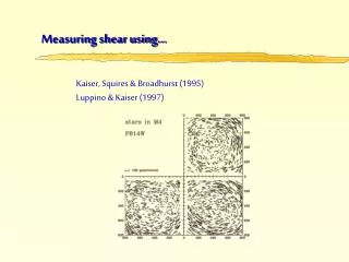
Measuring shear using… Kaiser, Squires & Broadhurst (1995) Luppino & Kaiser (1997)
Definition of shape If we have an object with axis ratios a and b: Ellipticity: e = 1 - b / a Polarisation: e = (a2-b2) / (a2+b2) Shear/stretch/distortion: g = (a-b) / (a+b) These are equivalent, but often called the wrong name
Quantifying shapes Many techniques quantify galaxy shapes in terms of the quadrupole moments of the image f And combine them into the spin-2 polarisation and The weight function W(q) is necessary because of noise. We use a Gaussian with a dispersion rg matched to the size of the galaxy.
How to obtain the “real” shape? Galaxies are typically convolved with an anisotropic point spread function. We also introduced a weight function. How do undo their effects? “Brute force” deconvolution of the galaxy deals with PSF anisotropy and size at the same time Approximate the problem (e.g., KSB95) Separates PSF anisotropy and size correction Each has its own advantages/disadvantages
Shear polarisability The first order shift in polarisation due to a shear is where the shear polarisability is given by a combination of higher order moments of the “true” image This tensor is close to diagonal and the diagonal terms are similar. Choice #1: Can we use the observed image? Choice #2: Use diagonal terms or full tensor?
How to deal with the PSF? = KSB assumption: PSF is convolution of a an istotropic function and a compact anisotropic function. Choice #3: Do we believe this?
In KSB the correction for PSF anisotropy and the size of the PSF are separated. The former is a shift in polarisation and the latter a rescaling. The anisotropic PSF changes the quadrupole moments qlm are the unweighted quadrupole moments of the PSF and Wlmij depend on higher order moments of the galaxy light distribution. Correction for PSF anisotropy
Correction for PSF anisotropy The shift in polarisation due to PSF anisotropy is The smear polarisability is a combination of higher order moments: and Choice #4: Use diagonal terms or full tensor?
Correction for PSF anisotropy PSF unweighted moments are not useful in practice… But the correction should work for stars are well, which should have zero polarisation after correction. So an alternative choice is to assume Choice #5: Use this assumption?
Correction for PSF anisotropy pa depends on the width of the adopted weight function; with the width matched to the size of the object, we “see” different parts of the PSF Choice #6: Which weight function to use?
Correction for PSF anisotropy KSB Unweighted PSF H98 Hoekstra et al. (1998): size matters…
Correction for PSF anisotropy Hoekstra et al. (1998)
Correction for PSF size Luppino & Kaiser showed how in the KSB formalism one can rescale the anisotropy corrected polarisations to obtain the `pre-seeing’ shear. with Choice #7: Which weight function to use? Choice #8: Use diagonal terms or full tensor?
Correction for PSF size LK97 H98 Hoekstra et al. (1998)
Correction for PSF size The pre-seeing shear polarisability is a noisy quantity for an individual object. It depends on the galaxy size, profile and shape. To reduce noise, one can average the values of galaxies with similar properties or use the ‘raw’ values. Choice #9: How does one implement this?
How to deal with noise? The images contain noise. Hence the polarisation of each galaxy has an associated measurement error. Hoekstra et al. (2000) showed how this can be estimated from the data. The noise estimate depends on higher order moments of the image. In addition the noise adds a small bias in the polarisation and polarisabilities because only the quadropole moments are linear in the noise. Choice #10: Should we correct for noise bias?
How to deal with noise? The pre-seeing shear polarisability approaches zero for objects that are comparable in size to the PSF. Noise in the polarisation is enhanced by a factor 1/Pg. Also residual systematics are scaled by this factor. We need to weight galaxies accordingly. The obvious choice is to use the inverse variance of the shear: Choice #11: Should we use this weighting?
How to deal with noise? By coincidence, the scatter in the polarisation is almost constant with apparent magnitude, but at the faint end one effectively measures noise. This becomes even more apparent when looking at the shear after correction for the size of the PSF.
How to deal with noise? We should also use “effective” source densities
How to deal with noise? A proper weighting should also account for the fact that more distant galaxies are lensed more efficiently. Hence, we need to modify the source redshift distribution to account for the weighting scheme.
Conclusions There are many choices on can make in the implementation of KSB. Although not always well defined, most choices are fairly obvious, or result in only minor differerences. The underlying assumption regarding the PSF appears silly, but remember that we are interested in ensemble averages. The ensemble averaged galaxy is close to a “Gaussian” and higher order effects tend to be averaged out due to the random orientation of galaxies. KSB is wrong for any given galaxy, but appears to do quite well in the ensemble average.


![Shear Force and Bending Moment Diagrams [SFD & BMD]](https://cdn3.slideserve.com/6594612/shear-force-and-bending-moment-diagrams-sfd-bmd-dt.jpg)