Describing Where: spatial referencing systems
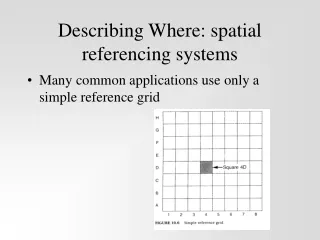
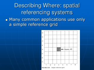
Describing Where: spatial referencing systems. Many common applications use only a simple reference grid. Rectangular referencing systems. Are not tied to spatial locations Often CAD drawings or scanned images suffer from this sort of referencing system

Describing Where: spatial referencing systems
E N D
Presentation Transcript
Describing Where: spatial referencing systems • Many common applications use only a simple reference grid
Rectangular referencing systems • Are not tied to spatial locations • Often CAD drawings or scanned images suffer from this sort of referencing system • There must be a way to tie the grid to specific places on earth
Geographic coordinates (Latitude and Longitude). Simple conversion of angles at the earth’s center gives a basic equirectangular projection Common and simple*
the Babylonian system is based on the number 60. Latitude and Longitude are based on a a "sexagesimal" system. A circle has 360 degrees, a degree has 60 min. and each minute is divided into 60 seconds. This nomenclature is known as DMS (degrees, minutes, seconds) • Perhaps a better system is to convert the minutes/seconds to a decimal part of a degree this is known as DD (decimal degrees). e.g. 120 30’ 00” = 120.5
A complicating factor: the Earth is not really ‘round’. It is in fact an ‘oblate spheroid’*.
Actually, the earth could be better pictured as a ‘lumpy potatoe’(my tribute to Dan Quayle) spinning through space. The Mathematical sphere and ellipsoid (sphereoid) are still open to “interpretation”
The picture is yet a little MORE complex! Not only do we have a lumpy blob of a planet, and we have to assume some mathematical construct to calculate locations We have to define WHERE the sphereoid is centered! http://www.connect.net/jbanta/FAQ.htmlAn outstanding site that discusses sphereoid and datum
Datum • The easiest to use are datum that use the center of the earth (WGS80,NAD84,GRS80) • Older data in the US often use NAD27 (North American Datum 1927). The datum for this projection is the geographic center of the conterminous US (Meads Ranch KS) • The offset between the same projection using a different datum can be significant • If you are aware of the issue, it is usually fairly easy to find the tools to make the conversion
While the Earth is ‘roundish’, maps/display screens are FLAT Map Projections are different ways that a curved surface can be displayed FLAT.
Continents drawn on oranges and made into a ‘flat’ maps... Ripping, tearing and distortion
Several projections do ‘interrupt’ the earth The Goode interrupted Homolosine equal-area projection The Cahill Butterfly projection (equal-area variant) The Schjerning equal-area projection for the oceans
Distortion: It is impossible to project a curved surface to a flat display without causing distortion of the features. An almost unlimited number of projections have been developed for the purposes of individual users. http://erg.usgs.gov/isb/pubs/MapProjections/projections.html http://www.colorado.edu/geography/gcraft/notes/mapproj/mapproj.html
A projection can intersect the surface in many different places. There is no distortion at the points of intersection… distortion increases as the distance from the intersecting points increases.
Handling Projections... • There are an almost unlimited number of ways that spatial data can be projected. • The most common in the US are probably: • Lat-long (geographic) • UTM (universal transverse mercator) • “State-Plane” with all that entails • “Albers” or “Lambert” conic projections
You must be aware that there are lots of possibilities You must know the terms. Be prepared, data almost NEVER overlays the first time. Never hesitate to look for help…
The direction of projection can be changed according to the needs of the person using the data
The UTM Grid (Universal Transverse Mercator) Projection Each Cell is 6 degrees of longitude and 8 degrees of latitude.
UTM zones for the Conterminous US: Note that most states are split between 2 or 3 zones… it is critical to know which zone your data are in. Nevada is one of the few states where virtually all state data are found in UTM coordinates.
UTM coordinates “read right, up” Report: Zone (e.g. 16 for AL) “eastings” (X) f then “northings”(Y)
Advantages of UTM • Values are always positive (a ‘false easting of 500,000 meters) • Equator 0 (all positive to the north) • South zone south pole is 0 all values are positive • Global coverage • High accuracy (meter by meter) • http://geology.isu.edu/geostac/Field_Exercise/topomaps/utm.htm
The “State Plane” Coordinate System • Each state has a unique set of coordinates • ‘wide’ states use a Lambert projection • ‘tall’ states use UTM projection • Larger states have multiple zones • The goal is to create minimal distortion between the curved surface and flat display and to have simple, positive coordinates
Wisconsin has 3 zones and uses a Lambert conic projection. Oregon has 2 zones and also uses the Lambert projection. Illinois uses a UTM projection
http://www.cnr.colostate.edu/class_info/nr502/lg3/datums_coordinates/spcs.htmlhttp://www.cnr.colostate.edu/class_info/nr502/lg3/datums_coordinates/spcs.html
Public Land Survey System • The idea of Thomas Jefferson • Set up in 1785 for the ‘western’ US • Creates ‘square’ landuse patterns. • Commonly used in parcel descriptions
SPSS baselines for the US… note the patterns of history and politics evident in the locations of PLSS.
Land use patterns in Ohio from Public Land Survey System (PLSS) survey. Land use patterns in Ohio from ‘uncontrolled’ survey.
Tennessee Alabama Roads from US Census TIGER files
N-S divisions are ‘TOWNSHIPs’ E-W divisions are ‘RANGE’ Each section is 1 mile square (640 Acres) The various ‘homestead’ acts gave rights of claim to a ¼ section…160 acres. 1 mile = .6km 1hectare = 2.2 acres
Projection...Coordinate System • Each projection has its own coordinate system and equations • Embedded in the software are the equations for each projection/datum • Projecting data is as simple as picking the correct sets of equations and ‘mashing the button’
Equations Embedded in the software Datam transformation
ArcGIS and Projections... • Projection information is defined in the data frame. • The first data layer in the data frame defines the project for subsequent layers... If the projection is defined for a data layer, Arc Map projects ‘on the fly’ and all layers overlay automatically • METADATA!! • These techniques do not work with poorly defined or undefined data
‘On the Fly’ projection • Takes time and computing power to redraw the map each time as every layer has to be projected to the data frame properties • DOES NOT CHANGE THE BASE DATA • Visual change only... • If the data are not accurately defined ‘on the fly’ projection will simply produce additional errors! In Arcview ..changing “view properties”
Dealing with projections.... • By far the best procedure is to use a standardized projection for all data in a project • This is not often a choice... Agencies choose the standard projection • Raster data (images) are much more complex to project, often it is best to match projection of vector data to the available raster data • Pick the projection for most of the data
COORDINATE SYSTEM DESCRIPTION THE Projection defined for Oregon GIS Data
The ArcGIS toolbox Define Projection allows you to specify the projection... Make sure you are correct! Project and Transform actually project the data (change the coordinates of the data) YOU MUST KNOW: What is the projection of the data now AND What the projection is that you wish to convert the data to
In Arcview.... • The ‘projection wizard’ is standard from V3.2 on • Available in the extensions pull down • SLOW......and has strange assumptions
Arcview Projection wizard • difficult to customize projection parameters, has a huge list of projections that are extremely uncommon... Standard projections are difficult to find
Explore the list ... Note that a LOT of projections are available... But they are not exactly what one might call ‘common’... Aside from some limitations it works well and it was a good first step towards what ArcGIS now uses
Projector! • In some ways a much superior tool for projecting data ... Much like the projection GUI in ArcToolbox • Comes with the SAMPLE extensions in Arcview... Its there, but ESRI does not tell you its there! • HOW to deal with extensions in Arcview 3.X
Lifting the hood ..... • Arcview extensions live in the ext32 directory
To make an extension active... • Simply copy the *.avx to the /ext32 directory • Turn on the check box in the extension menu and you are ready to rock • Demo... Projector!
In the sample extensions folder find the projector.avx file Copy this file to the ext32 directory Activate the PROJECTOR! extension
Added to the standard GUI is a new button for the Projector! extension