VII. References
Fiber-optic distributed temperature sensing network deployed in Waquoit Bay, MA (courtesy of USGS). Longitudinal temperature profile of Shenandoah River, VA (courtesy of USGS). Steelhead, Turtles, and Frogs: Temperature Dynamics of Stream Habitat

VII. References
E N D
Presentation Transcript
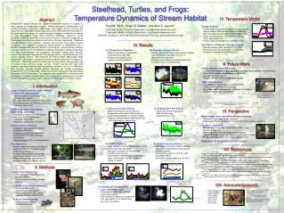
Fiber-optic distributed temperature sensing network deployed in Waquoit Bay, MA (courtesy of USGS) Longitudinal temperature profile of Shenandoah River, VA (courtesy of USGS) Steelhead, Turtles, and Frogs: Temperature Dynamics of Stream Habitat Paul M. Rich1, Stuart B. Weiss2, and Alan E. Launer3 1Creekide Center for Earth Observation, paul@creeksidescience.com 2Creekside Center for Earth Observation, stu@creeksidescience.com 3Stanford University, Land Use and Environmental Planning, aelauner@stanford.edu Abstract Availability of stream habitat with suitable temperature regimes is required by many species of conservation concern. Water temperature is determined by a complex interplay of prevailing meteorology, local riparian canopy structure and solar exposure, streambed morphology, and surface and subsurface flow patterns. We developed a technique for spatial-temporal analysis of temperature regimes for San Francisquito Creek (San Francisco Peninsula, California), which comprises habitat for steelhead (Oncorhynchus mykiss), California red-legged frog (Rana aurora draytonii) and western pond turtle (Clemmys marmorata). Steelhead requires relatively cool conditions, whereas the frog and turtle require warmer conditions. Our approach synthesized measurements of temperature from a network of inexpensive sensors (IButton Thermochron), riparian canopy structure and solar exposure from hemispherical (fisheye) photography, stream morphology from field characterization and geographic information system (GIS) analysis, stream flow and water temperature from gauging stations, and meteorology from nearby weather stations. We employed the RTemp Model (Washington State Department of Ecology) to predict time series of water temperature in response to heat fluxes. Water temperature co-varied with air temperature, diurnally with a lag of several hours, and over longer periods. Stream reaches with high solar exposure displayed relatively high temperature variability (up to 5° C differential from baseline), whereas shaded reaches displayed only modest temperature variability (0.5-1.0° C differential). Subsurface flow through gravel beds decreased temperature (2-3° C decrease). Our approach can be applied to a broad spectrum of streams for habitat characterization, for conservation management to ensure habitat heterogeneity, and for examination of potential impacts of climate change. IV. Temperature Model • Energy Balance • Predict water temperature based on energy balance using modified rTemp model (State of Washington, http://www.ecy.wa.gov/programs/eap/models.html) • Inputs: air temperature, solar radiation, canopy cover, water depth, etc. • Output: water temperature as a function of time • Simulation of Riparian Canopy Change • Riparian canopy cover varied from 0 to 100% • Increased solar exposure leads to proportional increase in daytime water temperature III. Results • Temperature Regimes • Water temperature co-varies with air temperature, with lags • Variance explained by solar exposure and flow patterns • B) Riparian Canopy Effects • Stream reaches with high solar exposure display high temperature variability (up to 5° C differential from baseline) • Shaded reaches display modest temperature variability (0.5–1.0° C differential) V. Future Work • Characterization and Modeling • Complete hemispherical photography and temperature sensor characterization • Characterize stream morphology (collaborationwith Balance Hydrologics) • Develop comprehensive temperature model • New Technologies • Use LIDAR for riparian canopy characterization(collaboration with Stanford/Carnegie) • Apply fiber-optic technique for distributed temperature sensing (collaboration with USGS) I. Introduction • Goal: Conserve species with different temperature requirements • Cooler temperature: Steelhead Trout (Oncorhyncus mykiss) • Warmer temperature: Northern red-legged frog (Rana aurora) and Western pond turtle (Clemmys marmorata) • Study Area: San Francisquito Watershed, California • Headwaters in Santa Cruz Mountains, drains into San Francisco Bay (37°27’ N, 120°00’ W) • 123 sq km, 3 tributaries, 24 creeks • Conservation Concerns • Changes in solar exposure: riparian vegetation modification • Changes in runoff / flow: watershed development and stream channel modification • Climate change: shifts in energy balance • Our Approach • Develop sampling protocol and energy balance model to characterize water temperature dynamics • Analyze relationships between solar exposure and temperature regimes • Relate temperature heterogeneity tohabitat suitability for different species • C) Diurnal Canopy Effects • Water temperature closely tracks air temperature when direct solar exposure • Lower diurnal variation in heavily shaded reaches, and peak water temperature lags >4 hr after peak air temperature • D) Subsurface Flow Effects • Subsurface flow through gravel beds can decrease temperature 2 - 3° C VI. Perspective • Water temperature key determinant of habitat • Steelhead Trout prefer cooler conditions • Red-Legged Frogs and Western Pond Turtles prefer warmer conditions • Synthetic Approach • Monitoring of flow, water temperature, meteorology, geomorphology, etc. • Solar exposure from hemispherical photographs • Observed temperature from Thermochron sensor network • Predicted temperature from energy balance model • Applicable for broad spectrum of streams • E) Solar Exposure • Solar radiation from hemiphotos every 2.5 m along 100 meter transects • Insolation increases >3-fold between October and June/July • Less riparian vegetation for “Dennis Martin” than “Lunar Rocks” reaches, leading to higher insolation • F) Spatial Autocorrelation • Spatial autocorrelation used to calculate appropriate hemispherical photography sampling interval • Semivariance peaks at 10-15 m, with pseudoperiodicity • Implication: sample interval of 10-20 m VII. References Danehy, R.J., et al. 2005. Patterns and sources of thermal heterogeneity in small mountain streams within a forested setting. Forest Ecology & Management 208:287-302. Fellers, G.M., et al. 2001. Overwintering tadpoles in the California Red-Legged Frog (Rana aurora draytonii). Herpetological Review 32:156-157. Johnson, S.L. 2004. Factors influencing stream temperatures in small streams: substrate effects and a shading experiment. Canadian Journal of Fisheries and Aquatic Sciences 61:913-923. Malcolm, I.A., et al. 2004. The influence of riparian woodland on the spatial and temporal variability of stream water temperatures in an upland salmon stream. Hydrology and Earth System Sciences 8:449-459. Moore, R.D., D.L. Spittlehouse, and A. Story. 2005. Riparian microclimate and stream temperature response to forest harvesting: A review. Journal of the American Water Resources Association 41:813-834. Rich, P.M. 1990. Characterizing plant canopies with hemispherical photography. Remote Sensing Reviews 5:13-29. Ringold, P.L., et al. 2003. Use of hemispheric imagery for estimating stream solar exposure. Journal of the American Water Resources Association 39:1373-1384. II. Methods • Long-Term Monitoring • Flow and water temperature from gauging stations • Meteorology from nearby weather stations • Intensive Field Measurements • Solar exposure using hemispherical photography • Water temperature using sensor network of iButton Thermochrons • Analysis and Modeling • Spatiotemporal patterns • Temperature model VIII. Acknowledgements • G) Simulated Tree Removal • Large California bay laurel (Umbellularia californica) removed using image editing • Tree removal increased solar exposure 2-3x, with effects 7.5 m downstream and 12.5 m upstream • Nina Allmendinger • Linda Chamberlin • Nona Chiariello • Trevor Hébert • Ryan Navratil • Bijan Osmani • Brian Scoles • Pam Sturner • Jasper Ridge Biological Preserve • National Fish and Wildlife Foundation • San Francisquito Watershed Council • Stanford University, Land Use and Environmental Planning Creek monkeys