Lab 4. Calculate <x> by Metropolis Monte Carlo method
230 likes | 478 Vues
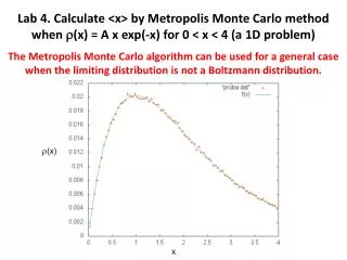
Lab 4. Calculate <x> by Metropolis Monte Carlo method when (x) = A x exp (-x) for 0 < x < 4 (a 1D problem). T he Metropolis Monte Carlo algorithm can be used for a general case when the limiting distribution is not a Boltzmann distribution. r (x). x.

Lab 4. Calculate <x> by Metropolis Monte Carlo method
E N D
Presentation Transcript
Lab 4. Calculate <x> by Metropolis Monte Carlo method when (x) = A x exp(-x) for 0 < x < 4 (a 1D problem) The Metropolis Monte Carlo algorithm can be used for a general case when the limiting distribution is not a Boltzmann distribution. r(x) x
Metropolis Monte Carlo Molecular Simulation (Review) state k Almost always involves a Markov process Move to a new configuration from an existing one according to a well-defined transition probability Simulation procedure 1. Generate a new “trial” configuration by making a perturbation to the present configuration. 2. Accept the new configuration based on the ratio of the probabilities for the new and old configurations, according to the Metropolis algorithm. 3. If the trial is rejected, the present configuration is taken as the next one in the Markov chain. 4. Repeat this many times, accumulating sums for averages. state k+1 David A. Kofke, SUNY Buffalo
Choices of Metropolis for canonical ensembles (review) N. Metropolis et al. J. Chem. Phys. 21, 1087 (1953) 1. Detailed balance condition • Symmetric : • Limiting probability distribution for canonical ensemble = Boltzmann • Transition probability & acceptance probability acc should satisfy: 4. Define the acceptance probability as: naturally satisfies this condition. Accept uphill moves only when not too uphill. • Accept all the • downhill moves.
Metropolis Monte Carlo algorithm for general cases 1. Detailed balance condition • Symmetric 3. Limiting probability distribution • Transition probability & acceptance probability acc should satisfy: naturally satisfies this condition. 4. Define the acceptance probability as: Accept moves toward less probable state according to the probability ratio (< 1). • Accept all the moves toward more probable state.
Displacement trial move. 1. Specification (Review) For a new configuration of the same volume V and number of molecules N, displace a randomly selected atom to a point chosen with uniform probability inside a cubic volume of edge d centered on the current position of the atom. Step 1 Step 2 Step 3 Step 4 Select an atom at random. Consider a region centered at it. Move atom to a point chosen uniformly in region. Consider acceptance of new configuration. ? general hitherto Examine underlying transition probability to formulate the acceptance criterion d David A. Kofke, SUNY Buffalo
Lab 4. Calculate <x> by Metropolis Monte Carlo method when (x) = A x exp(-x) for 0 < x < 4 (a 1D problem) mc: Metropolis MC code input - x0 : initial position of the particle (initial microstate) - n_steps: number of MC steps - n_thermo: frequency with which we write the observables (here: x, x2) - displ_max: maximum allowed displacement of the particle during a trial move - seed : random number generator seed - block_size: size of data block to perform statistics on the observables (x, x2) output files: - x.dat (position of the particle, text file) - x.bin (position of the particle, binary file - x2.dat (squared position of the particle, text file) (ignore for now)
mc.c (part 1) int main(int argc, char *argv[]) { int i, j, i_step, n_steps, n_thermo; double x0, k, temp, displ_max, x, pot_energy; double *x_b, *x2_b, x_avg, x2_avg; long seed; int block_size, n_blocks, i_block; int n_trial, n_accept; FILE *fp, *fp2, *fp3, *f_order; /* Get command-line input */ if (argc != 7) { fprintf(stderr, "Usage: %s x0 n_steps n_thermo displ_max seed block_size\n", argv[0]); exit(1); } x0 = atof(argv[1]); n_steps = atoi(argv[2]); n_thermo = atoi(argv[3]); displ_max = atof(argv[4]); seed = atoi(argv[5]); block_size = atoi(argv[6]); k = 1.0; temp = 1.0; (Ignore for now or use 1 for the block size.)
mc.c (part 2) /* Compute number of blocks and allocate memory */ if (n_steps % block_size != 0) { printf("n_steps must be a multiple of block_size\n"); exit(1); } n_blocks = n_steps / block_size; x_b = (double *) allocate_1d_array(n_blocks, sizeof(double)); x2_b = (double *) allocate_1d_array(n_blocks, sizeof(double)); /* Initialize block data */ for (i = 0; i < n_blocks; ++i) { x_b[i] = 0.0; x2_b[i] = 0.0; } /* Initialize variables for MC optimization. */ n_trial = 0; n_accept = 0; /* Open thermodynamic file. */ fp2 = fopen("x.dat", "w"); fp3 = fopen("x2.dat", "w"); f_order = fopen("x.bin", "w"); (Ignore for now or use 1 for the block size.)
mc.c (part 3 – main MC loop) /* MC loop. */ i_block = 0; x = x0; /* x0 corresponds to the initial microstate. */ for (i_step = 1; i_step <= n_steps; ++i_step) { /* Perform a MC cycle. */ mc_cycle(&x, displ_max, temp, k, &seed, &pot_energy, &n_trial, &n_accept); /* Write thermodynamic quantities in file every cycle. */ if (i_step % n_thermo == 0) { fprintf(fp2, "%d %12.8f\n", i_step, x); fprintf(fp3, "%d %12.8f\n", i_step, x*x); fwrite(&x, sizeof(double), 1, f_order); } /* Block accumulation. */ x_b[i_block] += x; x2_b[i_block] += x*x; /* Block average. */ if (i_step % block_size == 0) { x_b[i_block] /= (double) block_size; x2_b[i_block] /= (double) block_size; printf("bloc %d: x = %12.8f, x2 = %12.8f\n", i_block, x_b[i_block], x2_b[i_block]); printf("----------------------------------\n"); ++i_block; } } (Ignore for now or use 1 for the block size.)
mc_cycle.c /* This routine carries out a single Monte Carlo cycle, comprising only of Monte Carlo atom move. Output: particle positions and potential energy are modified on output */ #include "test.h" #include "mc_cycle.h" #include "atom_move.h" void mc_cycle(double *x, double displ_max, double temp, double k, long *seed, double *u_pot, int *n_trial, int *n_accept) { int i_move; /* Make trial move. */ ++(*n_trial); *n_accept += atom_move(x, displ_max, temp, k, seed, u_pot); return; }
atom_move.c /* This routine generates a trial displacement of an interaction atom and accepts it based on the Metropolis criterion. Output: the return value is 1 if the move was accepted and 0 otherwise. */ #include "test.h" #include "atom_move.h" #include "ran3.h" int atom_move(double *x, double displ_max, double temp, double k, long *seed, double *u_pot) { int accept; double p_old, p_new, delta_p; double displ, x_old; x_old = *x; p_old = x_old * exp(-x_old); /* Generate random displacement within hypercube of size displ_max. */ displ = displ_max * (ran3(seed) - 0.5); *x += displ; /* Compute change in potential energy and accept move using Metropolis criterion. */ if (*x > 4.0 || *x < 0.0) p_new = 0.0; else p_new = (*x) * exp(-(*x)); delta_p = p_new / p_old; if (delta_p >= 1.0) accept = 1; else accept = ran3(seed) < delta_p; /* Update system potential energy if trial move is accepted. Otherwise, reset variables. */ if (!accept) { *x = x_old; } /* Return 1 if trial move is accepted, 0 otherwise. */ return accept; } Consider a region of (displ_max) centered at x_old to choose x_new. (1-body 1-dimension case)
Displacement trial move. 1. Specification (Review) For a new configuration of the same volume V and number of molecules N, displace a randomly selected atom to a point chosen with uniform probability inside a cubic volume of edge d centered on the current position of the atom. Step 1 Step 2 Step 3 Step 4 Select an atom at random. Consider a region centered at it. Move atom to a point chosen uniformly in region. Consider acceptance of new configuration. ? general hitherto Examine underlying transition probability to formulate the acceptance criterion d David A. Kofke, SUNY Buffalo
Metropolis Monte Carlo algorithm for general cases 1. Detailed balance condition • Symmetric 3. Limiting probability distribution • Transition probability & acceptance probability acc should satisfy: naturally satisfies this condition. 4. Define the acceptance probability as: Accept moves toward less probable state according to the probability ratio (< 1). • Accept all the moves toward more probable state.
Analysis 1 (Tools are provided in a subdirectory analysis.) 1) mean_sample: computes the sample mean of x and compare to the exact value. input: - x.dat or x.bin (output from mc) - ascii: read the .dat file (1) or read the .bin file (0) output: - mean value - sample mean and with (integration by parts) 2) hist: calculates the histogram of x (i.e the probability to find x in [0,4]). input: - x.dat or x.bin (output from mc) - ascii: read the .dat file (1) or read the .bin file (0) - n_bins: number of bins in the histogram, each bin having a size: output: - hist.dat: the histogram file with elements i.e. probability to find the particle at position x in [xi, xi + Dx]
D = 0.5 (Pacc = 95%, <x> = 1.6731) 1000 consecutive x values of Markov chain for different step sizes () among the total number of values or steps M = 2106 D = 8 (Pacc = 37%, <x> = 1.6760)) • = 200 (Pacc = 1.5%, <x> = 1.6701)
Histogram of x values for = 8 & a fit with(x) = A x exp(-x) r(x) x
Correlation is significant for = 0.5 and 200 and negligible for = 8.
Analysis 2 (Tools are provided in a subdirectory analysis.) 3) time_corr: calculates correlation time using autocorrelation function C(k) (single time origin) input: - x.dat or x.bin (from mc) - ascii: read the .dat file (1), read the .bin file (0) - k_max: maximum separation between data considered to evaluate time correlation output: - time_corr.dat: time correlation function C(k) - time_integrated.dat: the integrated correlation time t(k) 4) block: calculates correlation time using block method (successive blocks of size 2n, n = 0,..,16) for n = 1: New serie with M/2 values (block size 21) for n = k : new serie with M/2k values (each value is a block of size 2k) input: - x.dat or x.bin (output from mc) - ascii: read the .dat file (1) or read the .bin file (0) output: - block.dat: uses columns 1 (n) and 8 (correlation time)
Example of data correlation: 1D harmonic oscillator (review) Autocorrelation functions for the complete data sets (400,000 steps) of x for three different step sizes = 1; 10; 200 (acceptance rate = 0.70; 0.35; 0.02) (fluctuation around the average), where which measure whether the fluctuations are related for x values l measurement apart. e-1 correlation time (long) correlation time (short) correlation time (long) In generating these results so far, x was measured every MC step.
Autocorrelation function & Integrated correlation time tint Accumulated tint Autocorrelation function C(k) k k
Block Method correlation time t k (block size = 2k)