Lightning Forecast Algorithm: Enhancing Storm Prediction
Implementing a lightning forecast algorithm using WRF simulations for accurate peak flash rate densities. Comparison of CAPE vs LFA coverage and methodology insights.

Lightning Forecast Algorithm: Enhancing Storm Prediction
E N D
Presentation Transcript
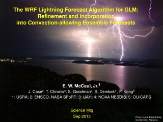
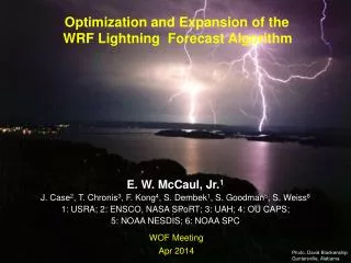
Lightning Forecast Algorithm (R3) E. W. McCaul, Jr. USRA Huntsville High Impact WW Feb 24, 2011 Photo, David Blankenship Guntersville, Alabama
Objectives Given LTG link to large ice, and a good CRM like WRF, we seek to: Create WRF forecasts of LTG threat (1-24 h), based on simple proxy fields from explicitly simulated convection: - graupel flux near -15 C (captures LTG time variability) - vertically integrated ice (captures anvil LTG area) Construct a calibrated threat that yields accurate quantitative peak flash rate densities for the strongest storms, based on LMA total LTG data 3. Test algorithm over CONUS to assess robustness for use in making proxy LTG data, potential uses with DA
WRF Lightning Threat Forecasts:Methodology Use high-resolution 2-km WRF simulations to prognose convection for a diverse series of selected case studies Evaluate two proxy fields: graupel fluxes at -15C level; vertically integrated ice (VII=cloud ice+snow+graupel) Calibrate these proxies using peak total LTG flash rate densities from NALMA vs. strongest simulated storms; relationships ~linear; regression line passes through origin 4. Truncate low threat values to make threat areal coverage match NALMA flash extent density obs Blend proxies to achieve optimal performance 6. Study NSSL 4-km, CAPS 4-km CONUS ensembles to evaluate performance, assess robustness
WRF Lightning Threat Forecasts:Methodology Regression results for threat 1 “F1” (based on graupel flux FLX = w*qg at T=-15 C): F1 = 0.042*FLX (require F1 > 0.01 fl/km2/5 min) Regression results for threat 2 “F2” (based on VII, which uses cloud ice + snow + graupel from WRF WSM-6): F2 = 0.2*VII (require F2 > 0.4 fl/km2/5 min)
Calibration Curve Threat 1 (Graupel flux) F1 = 0.042 FLX F1 > 0.01 fl/5 min r = 0.67
Calibration Curve Threat 2 (VII) F2 = 0.2 VII F2 > 0.4 fl/5 min r = 0.83
Methods based on LTG physics; should be robust and regime-independent Can provide quantitative estimates of flash rate fields; use of thresholds allows for accurate threat areal coverage Methods are fast and simple; based on fundamental model output fields; no need for complex electrification modules LTG Threat Methodology: Advantages
Methods are only as good as the numerical model output; models usually do not make storms in the right place at the right time; saves at 15 min sometimes miss LTG jump peaks Small number of cases, lack of extreme LTG events means uncertainty in calibrations Calibrations should be redone whenever model is changed (see example next page; pending studies of sensitivity to grid mesh, model microphysics, to be addressed here) LTG Threat Methodology: Disadvantages
2-km horizontal grid mesh 51 vertical sigma levels Dynamics and physics: Eulerian mass core Dudhia SW radiation RRTM LW radiation YSU PBL scheme Noah LSM WSM 6-class microphysics scheme (graupel; no hail) 8h forecast initialized at 00 UTC 30 March 2002 with AWIP212 NCEP EDAS analysis; Also used METAR, ACARS, and WSR-88D radial vel at 00 UTC; Eta 3-h forecasts used for LBC’s WRF Configuration (typical)30 March 2002 Case Study
WRF Lightning Threat Forecasts:Case: 30 March 2002Squall Line plus Isolated Supercell
WRF Sounding, 2002033003Z Lat=34.4 Lon=-88.1 CAPE~2800
Ground truth: LTG flash extent density + dBZ30 March 2002, 04Z
WRF forecast: LTG Threat 2 + 10 km anvil ice30 March 2002, 04Z
Implications of results:1. WRF LTG threat 1 coverage too small (updrafts emphasized)2. WRF LTG threat 1 peak values have adequate t variability 3. WRF LTG threat 2 peak values have insufficient t variability (because of smoothing effect of z integration)4. WRF LTG threat 2 coverage is good (anvil ice included)5. WRF LTG threat mean biases can exist because our method of calibrating was designed to capture peak flash rates, not mean flash rates6. Blend of WRF LTG threats 1 and 2 should offer good time variability, good areal coverage
Construction of blended threat:1. Threat 1 and 2 are both calibrated to yield correct peak flash densities2. The peaks of threats 1 and 2 also tend to be coincident in all simulated storms, but threat 2 covers more area3. Thus, weighted linear combinations of the 2 threats will also yield the correct peak flash densities 4. To preserve most of time variability in threat 1, use large weight w15. To preserve areal coverage from threat 2, avoid very small weight w26. Tests using 0.95 for w1, 0.05 for w2, yield satisfactory results
General Findings:1. LTG threats 1 and 2 yield reasonable peak flash rates2. LTG threats provide more realistic spatial coverage of LTG than that suggested by coverage of positive CAPE, which overpredicts threat area, especially in summer - in AL cases, CAPE coverage ~60% at any t, but our LFA, NALMA obs show storm coverage only ~15% - in summer in AL, CAPE coverage almost 100%, but storm time-integrated coverage only ~10-30% - in frontal cases in AL, CAPE coverage 88-100%, but squall line storm time-integrated coverage is 50-80% 3. Blended threat retains proper peak flash rate densities, because constituents are calibrated and coincident4. Blended threat retains temporal variability of LTG threat 1, and offers proper areal coverage, thanks to threat 2
Ensemble studies, CAPS cases, 2008:(examined to test robustness under varying grids, physics)1. Examined CAPS ensemble output for two AL-area storm events from Spring 2008: 2 May and 11 May2. NALMA data examined for both cases to check LFA 3. Caveats based on data limitations: - CAPS grid mesh 4 km, whereas LFA trained on 2 km mesh - model output saved only hourly; no peak threats available - to check calibrations, use mean of 12 NALMA 5-min peaks4. Results from 10 CAPS ensemble members, 2 cases: - Threat 1 always smaller than Threat 2, usually 10-20% - Threat 2 values look reasonable compared to NALMA - Threat 1 shows more sensitivity to grid change than Threat 2
CAPS p2, Threat 1: 2008050300Z (Member p2 chosen for its resemblance to original WRF configuration)
CAPS p2, Threat 2: 2008050300Z (Note greater amplitude and coverage of Threat 2 vs. Threat 1)
Ensemble findings (preliminary):1. Tested LFA on two CAPS 2008 4km WRF runs2. Two cases yield consistent, similar results3. Results sensitive to coarser grid mesh, model physics - Threat 1 too small, more sensitive (grid mesh sensitivity?) - Threat 2 appears less sensitive to model changes - Remedy: boost Threat 1 to equal Threat 2 peak values before creating blended Threat 34. Implemented modified LFA in NSSL WRF 4 km runs in 2010
2010 work with NSSL WRF:1. LFA now used routinely on NSSL WRF 30-h runs2. See www.nssl.noaa.gov/wrf and look for Threat plots3. Results are expressed in terms of hourly gridded maxima for threats 1, 2, before rescaling of threat 1; units are flashes per sq. km per 5 min4. To make blended threat 3, we use fields of hourly maxima of threats 1,2, after appropriate rescaling of threat 15. Potential issues: in snow events, can have spurious threat 2; in extreme storms, threat 2 fails to keep up with threat 1, even though coarser grid argues for need to boost threat 1; further study needed6. NSSL collaborators, led by Jack Kain, tested LFA reliability against existing LTG forecast tools, with favorable findings
Sample of NSSL WRF output, 20101130 (see www.nssl.noaa.gov/wrf)
Scatterplot of selected NSSL WRF output for threats 1, 2 (internal consistency check) Threats 1, 2 should cluster along diagonal; deviation at high flash rates indicates need for recalibration
Future Work:1. Examine more simulation cases from 2010 Spring Expt; test LFA against dry summer LTG storms in w USA2. Compile list of intense storm cases, and use NALMA, OKLMA data to recheck calibration curves for nonlinear effects; test for sensitivity to additional storm parameters 3. Run LFA in CAPS 2011 ensembles, assess performance; - evaluate LFA in other configurations of WRF ARW - more hydrometeor species - double-moment microphysics4. LFA threat fields may offer opportunities for devising data assimilation strategies based on observed total LTG, from both ground-based and satellite systems (GLM)
Acknowledgments:This research was funded by the NASA Science Mission Directorate’s Earth Science Division in support of the Short-term Prediction and Research Transition (SPoRT) project at Marshall Space Flight Center, Huntsville, AL. Thanks to collaborators Steve Goodman, NOAA, and K. LaCasse and D. Cecil, UAH, who helped with the recent W&F paper (June 2009). Thanks to Gary Jedlovec, Rich Blakeslee, Bill Koshak (NASA), and Jon Case (ENSCO) for ongoing support for this research. Thanks also to Paul Krehbiel, NMT, Bill Koshak, NASA, Walt Petersen, NASA, for helpful discussions. For published paper, see:McCaul, E. W., Jr., S. J. Goodman, K. LaCasse and D. Cecil, 2009:Forecasting lightning threat using cloud-resolving model simulations. Wea. Forecasting, 24, 709-729.