Statistical Analysis Methods for Testing Population Parameters
200 likes | 222 Vues
Learn how to test if two populations' means or percentages are truly different using chi-squared tests. This unit covers sample selection, confidence intervals, hypothesis testing, and practical examples in various fields.

Statistical Analysis Methods for Testing Population Parameters
E N D
Presentation Transcript
Testing %’s of 2 populations: equal? • Take a sample from each population; theirx’s (or %’s) won’t be equal. Are they different enough to say populations’μ’s (or %’s) are unequal? • Fact: SE of difference in sample avgs from two populations is √[(SE1)2 + (SE2)2] • So for CI of diff in %: • SE of diff = √[p1(1-p1)/n1 + p2(1-p2)/n2] where • p’s are samples’ %’s & n’s are sample sizes • (… assuming n’s are big enough for z-test) • For sig test of diff in %, H0 : %’s are = ; bootstrap for common population % with “pooled estimate” p = (n1p1 + n2p2)/(n1+n2), : • SE = √[p(1-p)(1/n1 + 1/n2)]
Example: NYRI • In Morrisville, a sample of 100 people shows 65% against NYRI. In Hamilton, a sample of 150 is 60% against. Is NYRI more unpopular in Morrisville than Hamilton? • SE for CI: √[.65(.35)/100+.6(.4)/150] ≈ 6.22% • so 95% CI is 65% ± 2(6.22%) • which includes 60% • SE for z-test: “pooled” p = (.65(100)+.6(150)) / (100+150) = .62 • so SE is √[.62(.38)(1/100+1/150)] ≈ 6.26% • so z = (5%-0%)/6.26% ≈ .80, not significant diff
Example: prenatal AZT • Does giving the drug AZT to HIV-positive pregnant women save their babies from HIV? (Newsweek, March 7, 1994, p. 53) Out of 163 babies born to mothers treated with AZT, only 13 were HIV-positive, while out of 161 born to mothers treated with a placebo, 40 were HIV-positive.
Testing μ’s (not %’s) of 2 populations: equal? • Difference ofx’s of two samples approximates difference of populations’ μ’s • The formula for SE of sample difference is now √[(s12/n1) + (s22/n2)] (bootstrapping) • If samples are small enough to need a t-test, the value for df is (a mess, but) ≥ min(n1-1,n2-1) (and usually near n1 + n2 – 2)
Example: better at math? • A standard math test is given to 25 randomly chosen Colgate students and 25 Hamilton College students. The Colgate students averaged 155 of a possible 200, with an SD of 15; the Hamilton students averaged 150, with an SD of 20. Are Colgate students better at math?
Example: OAEs • Is there a prenatal basis for homosexuality? (McFadden & Pasanen, Proc. Natl. Acad. Sci. USA, 95 (1998), 2709-2713) If a quiet click sound is made outside a person’s ear, the inner ear responds with “otoacoustic emissions” (OAEs), measured by a mic in ear canal. The inner ears of women usually generate stronger OAEs than men for same volume click (maybe because of androgens in womb). This study: Right ears of 57 heterosexual women produced OAEs of avg amplitude 18.2 dB SPL, with SE of 0.8 dB (in response to click of 75 dB); for 37 homosexual women, avg 16.0 and SE 0.7. Is the difference significant?
Example: Music lessons for math? Does music help a child learn math? (Inspired by Newsweek, July 24, 2000, pp. 50-52): One group of 26 second-graders gets piano instruction plus practice with a math video game; another group of 29 gets extra English lessons plus the math game. After four months, the first group gets an average score of 69 on a test of ratios and fractions, with an SD of 10, while the second averages 60, with an SD of 15.
χ2-tests for counts (I) • Given a list of frequencies (counts), are they distributed (significantly) differently from an expected list? • Or, given a table of frequencies, are the counts distributed (significantly) differently in different rows [or columns]? • I.e., does the choice of category represented by the row affect the distribution of the frequencies in the categories represented by the columns? • Or are the column categories “independent” of the row categories, and v.v.?
Ex of χ2-test: Admittance bias by HS? A certain college claims it does not use an applicant's high school as a factor in the decision to admit him/her. Does the following data support that claim?
χ2-tests for counts (II) • [Toy example: Frequencies are too small for true “asymptotic” test; all cells should have ≥ 5] • H0: % admitted would be same for all HSs • so expected = (22/75)(# applied) • χ2 = Σ (observed–expected)2/expected • If observed = expected, term would be 0 • Always ≥ 0 • Must be counts, not %’s or fractions (would change X2 value) • Here, = 2.69 • Useχ2-table with df = #cols – 1 = 6 • [ times (# rows – 1), which is 1 here ]
Ex of χ2-test: Family sizes & geography • A survey gives the following information on the numbers of children that couples have in different regions of the country. Are the differences between the regions due to chance?
Family size & geography, ctnd. • H0: distribution of family sizes is same all over. • expected = (row sum)(column sum)/(total) • χ2 = Σ(obs - exp)2/exp = 9.244 • df = (4-1)(3-1) = 6
So you’ve done a significance test and gotten significance. Now what? • It may still be just chance. • It may reflect bias in the experiment or study. • *It must reflect a box model with chance errors, even though the arithmetic doesn’t refer to it (as in a χ2 test) • *It may not be important, even if the use of a large sample makes a small significance level.
Type I and type II errors • A “type I” error in a sig test is to reject H0 when it is true. • Many “discoveries” are type I errors • By def, α-value is P(type I error | H0 is true) • A “type II” error is to fail to reject H0 when it is false. • We never “accept H0” – no science is exactly right. (E.g., Einstein corrected Newton.)
Example: α-level and type I or II Flip a coin, get 8 heads. With an H0 of a fair coin, P(count ≥ 8) = [C(10,8) + C(10,9) + C(10,10)] / 210≈ 5.5% So with α = 10%, we reject null, while with α = 5%, we do not reject null. • Therefore, if the coin is fair, 10% makes a type I error, and 5% yields the correct answer, • while if the coin is unfair, 10% yields the correct answer, and 5% makes a type II error.
The “power” of a test is P(no type II error | H0 is false) = 1 - P(type II | H0 false), but ... • ... we can’t compute the power because it depends on how false H0 is, and usually we don’t even know whether it is false. • Ex: Test a coin for fairness (H0 : P(head) = 0.5) with 20 flips. With α = 5%, test says coin unfair if #heads <= 5 or >= 15.Sample (binomial) distributions whenP(head) = 0.6 and 0.7: P(type II error) = 87% and 58% respectively.
Another example: An oracle speaks • Valesky vs. Brown for State Senate, interviewing 400 people. • H0: p = 50% of voters for Val; Ha: p > 50% • EV of (sample) % = .5, SE of % = √[.5(.5)/400] = .025 • For sig, need z = ((#/400)-.5)/.025 ≥ 1.96, i.e., # ≥ 220 • Oracle reveals true p = 52%: EV = .52, SE = √(.52(.48)/400) = .025 : P(Type II error) = P(z ≤ ((220/400)-.52)/.025 = 1.2) = 89% • Oracle reveals true p = 55%: EV = .55, SE = √(.55(.45)/400) = .025 : P(Type II error) = P(z ≤ ((220/400)-.55)/.025 = 0) = 50%
Still, … • As P(Type I error) [rejecting H0 when you shouldn’t] goes up -- maybe by picking a larger α or using a larger sample -- P(Type II error) [failing to reject H0 when you should] goes down, and v.v.