Properties of Random Number Generation Techniques
Learn about generating pseudo-random numbers, Linear Congruential Method, examples, characteristics of a good generator, and techniques for random variate generation. Dive into Inverse-transform and Discrete Distributions.

Properties of Random Number Generation Techniques
E N D
Presentation Transcript
Properties of Random Numbers • Random Number, Ri, must be independently drawn from a uniform distribution with pdf: • Two important statistical properties: • Uniformity • Independence. U(0,1) Figure: pdf for random numbers
Generation of Pseudo-Random Numbers • “Pseudo”, because generating numbers using a known method removes the potential for true randomness. • Goal: To produce a sequence of numbers in [0,1] that simulates, or imitates, the ideal properties of random numbers (RN). • Important considerations in RN routines: • Fast • Portable to different computers • Have sufficiently long cycle • Replicable • Closely approximate the ideal statistical properties of uniformity and independence.
Linear Congruential Method [Techniques] • To produce a sequence of integers, X1, X2, … between 0 and m-1 by following a recursive relationship: • The selection of the values for a, c, m, and X0 drastically affects the statistical properties and the cycle length. • The random integers are being generated [0,m-1], and to convert the integers to random numbers: The modulus The multiplier The increment
Examples[LCM] • Use X0 = 27, a = 17, c = 43, and m = 100. • The Xi and Ri values are: X1 = (17*27+43) mod 100 = 502 mod 100 = 2, R1 = 0.02; X2 = (17*2+43) mod 100 = 77, R2 = 0.77; X3 = (17*77+43) mod 100 = 52, R3 = 0.52; X4 = (17* 52 +43) mod 100 = 27, R3 = 0.27 • “Numerical Recipes in C” advocates the generator a = 1664525, c = 1013904223, and m = 232 • Classical LCG’s can be found on http://random.mat.sbg.ac.at
Characteristics of a Good Generator[LCM] • Maximum Density • Such that the values assumed by Ri, i = 1,2,…, leave no large gaps on [0,1] • Problem: Instead of continuous, each Ri is discrete • Solution: a very large integer for modulus m • Approximation appears to be of little consequence • Maximum Period • To achieve maximum density and avoid cycling. • Achieve by: proper choice of a, c, m, and X0. • Most digital computers use a binary representation of numbers • Speed and efficiency are aided by a modulus, m, to be (or close to) a power of 2.
A Good LCG Example X=2456356; %seed value for i=1:10000, X=mod(1664525*X+1013904223,2^32); U(i)=X/2^32; end edges=0:0.05:1; M=histc(U,edges); bar(M); hold; figure; hold; for i=1:5000, plot(U(2*i-1),U(2*i)); end
Randu (from IBM, early 1960’s) X=1; %seed value for i=1:10000, X=mod(65539*X+57,2^31); U(i)=X/2^31; end edges=0:0.05:1; M=histc(U,edges); bar(M); hold; figure; hold; for i=1:3333, plot3(U(3*i-2),U(3*i-1),U(3*i)); end Marsaglia Effect (1968)
Random-Numbers Streams[Techniques] • The seed for a linear congruential random-number generator: • Is the integer value X0 that initializes the random-number sequence. • Any value in the sequence can be used to “seed” the generator. • A random-number stream: • Refers to a starting seed taken from the sequence X0, X1, …, XP. • If the streams are b values apart, then stream i could defined by starting seed: • Older generators: b = 105; Newer generators: b = 1037. • A single random-number generator with k streams can act like k distinct virtual random-number generators • To compare two or more alternative systems. • Advantageous to dedicate portions of the pseudo-random number sequence to the same purpose in each of the simulated systems.
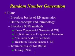
Purpose & Overview • Develop understanding of generating samples from a specified distribution as input to a simulation model. • Illustrate some widely-used techniques for generating random variates. • Inverse-transform technique • Convolution technique • Acceptance-rejection technique • A special technique for normal distribution 11
r = F(x) r1 x1 Inverse-transform Technique • The concept: For cdf function: r = F(x) • Generate R sample from uniform (0,1) • Find X sample: X = F-1(R) 12
Exponential Distribution [Inverse-transform] • Exponential Distribution: • Exponential cdf: • To generate X1, X2, X3 ,… generate R1, R2, R3 ,… r = F(x) = 1 – e-xfor x 0 Xi = F-1(Ri) = -(1/ ln(1-Ri) Figure: Inverse-transform technique for exp( = 1) 13
Exponential Distribution [Inverse-transform] • Example: Generate 200 variates Xi with distribution exp(= 1) • Matlab Code for i=1:200, expnum(i)=-log(rand(1)); end R and (1 – R) have U(0,1) distribution 14
Uniform Distribution [Inverse-transform] • Uniform Distribution: • Uniform cdf: • To generate X1, X2, X3 ,…, generate R1, R2, R3 ,… 15
Uniform Distribution [Inverse-transform] • Example: Generate 500 variates Xi with distribution Uniform (3,8) • Matlab Code for i=1:500, uninum(i)=3+5*rand(1); end 16
Discrete Distribution [Inverse-transform] All discrete distributions can be generated by the Inverse-transform technique. F(x) p1 + p2 + p3 p1 + p2 R1 p1 General Form b a c 17
Discrete Distribution [Inverse-transform] • Example: Suppose the number of shipments, x, on the loading dock of IHW company is either 0, 1, or 2 • Data - Probability distribution: • Method - Given R, the generation scheme becomes: Consider R1 = 0.73: F(xi-1) < R <= F(xi) F(x0) < 0.73 <= F(x1) Hence, x1 = 1 18
Convolution Technique • Use for X = Y1 + Y2 + … + Yn • Example of application • Erlang distribution • Generate samples for Y1 , Y2 , … , Yn and then add these samples to get a sample of X. 19
Erlang Distribution [Convolution] • Example: Generate 500 variates Xi with distribution Erlang-3 (mean: k/ • Matlab Code for i=1:500, erlnum(i)=-1/6*(log(rand(1))+log(rand(1))+log(rand(1))); end 20
Generate Y,U no Condition yes Output X=Y Acceptance-Rejection technique • Useful particularly when inverse cdf does not exist in closed form • a.k.a. thinning • Steps to generate X with pdf f(x) • Step 0: Identify a majorizing function g(x) and a pdf h(x) satisfying • Step 1: Generate Y with pdf h(x) • Step 2: Generate U ~ Uniform(0,1) independent of Y • Step 3: Efficiency parameter is c 21
Generate Y~U(0,0.5) and U~U(0,1) no yes Output X = Y Triangular Distribution [Acceptance-Rejection] 22
Triangular Distribution [Acceptance-Rejection] Matlab Code: (for exactly 1000 samples) i=0; while i<1000, Y=0.5*rand(1); U=rand(1); if Y<=0.25 & U<=4*Y | Y>0.25 & U<=2-4*Y i=i+1; X(i)=Y; end end 23
Poisson Distribution [Acceptance-Rejection] • N can be interpreted as number of arrivals from a Poisson arrival process during one unit of time • Then, the time between the arrivals in the process are exponentially distributed with rate
Poisson Distribution [Acceptance-Rejection] • Step 1. Set n = 0, and P = 1 • Step 2. Generate a random number Rn+1 and let P = P. Rn+1 • Step 3. If P < e-, then accept N = n. Otherwise, reject current n, increase n by one, and return to step 2 • How many random numbers will be used on the average to generate one Poisson variate?
Normal Distribution [Special Technique] • Approach fornormal(0,1): • Consider two standard normal random variables, Z1 and Z2, plotted as a point in the plane: • B2 = Z21 + Z22 ~ chi-square distribution with 2 degrees of freedom = Exp( = 1/2). Hence, • The radius B and angle are mutually independent. Uniform(0,2 In polar coordinates: Z1 = B cos Z2 = B sin 26
Normal Distribution [Special Technique] • Approach fornormal(,): • Generate Zi ~ N(0,1) • Approach for lognormal(,): • Generate X ~ N(,) Xi = + Zi Yi = eXi 27
Normal Distribution [Special Technique] • Generate 1000 samples of Normal(7,4) • Matlab Code for i=1:500, R1=rand(1); R2=rand(1); Z(2*i-1)=sqrt(-2*log(R1))*cos(2*pi*R2); Z(2*i)=sqrt(-2*log(R1))*sin(2*pi*R2); end for i=1:1000, Z(i)=7+2*Z(i); end 28