Mastering Divide and Conquer Algorithms: Mergesort, Quicksort
Explore the principles of divide and conquer algorithms such as Mergesort and Quicksort. Understand the Master Theorem for efficient problem-solving strategies. Learn to apply these concepts through practical examples and analyses. Enhance your understanding of binary search, binary trees, and more. Master the art of algorithm design with this comprehensive guide.


Mastering Divide and Conquer Algorithms: Mergesort, Quicksort
E N D
Presentation Transcript
The Design and Analysis of Algorithms Chapter 4:Divide and Conquer Master Theorem, Mergesort, Quicksort, Binary Search, Binary Trees
Chapter 4. Divide and Conquer Algorithms • Basic Idea • Merge Sort • Quick Sort • Binary Search • Binary Tree Algorithms • Closest Pair and Quickhull • Conclusion
Basic Idea • Divide instance of problem into two or more smaller instances • Solve smaller instances recursively • Obtain solution to original (larger) instance by combining these solutions
a problem of size n subproblem 1 of size n/2 subproblem 2 of size n/2 a solution to subproblem 1 a solution to subproblem 2 a solution to the original problem Basic Idea
General Divide-and-Conquer Recurrence T(n) = aT(n/b) + f (n)where f(n)(nd), d 0 Master Theorem:If a < bd, T(n) (nd) If a = bd, T(n) (nd log n) If a > bd, T(n) (nlog b a ) • Examples: T(n) = T(n/2) + nT(n) (n ) Here a = 1, b = 2, d = 1, a < bd T(n) = 2T(n/2) + 1T(n) (nlog 2 2) = (n ) Here a = 2, b = 2, d = 0, a > bd
Examples • T(n) = T(n/2) + 1T(n) (log(n) ) Here a = 1, b = 2, d = 0, a = bd • T(n) = 4T(n/2) + nT(n) (n log 2 4)= (n 2) Here a = 4, b = 2, d = 1, a > bd • T(n) = 4T(n/2) + n2T(n) (n2 log n) Here a = 4, b = 2, d = 2, a = bd • T(n) = 4T(n/2) + n3T(n) (n3) Here a = 4, b = 2, d = 3, a < bd
cn2 c(n/4)2 c(n/4)2 c(n/4)2 T(n/16) T(n/16) T(n/16) T(n/16) T(n/16) T(n/16) T(n/16) T(n/16) T(n/16) (c) Recursion Tree for T(n)=3T(n/4)+(n2) T(n) cn2 T(n/4) T(n/4) T(n/4) (a) (b) cn2 cn2 (3/16)cn2 c(n/4)2 c(n/4)2 c(n/4)2 log 4n (3/16)2cn2 c(n/16)2 c(n/16)2 c(n/16)2 c(n/16)2 c(n/16)2 c(n/16)2 c(n/16)2 c(n/16)2 c(n/16)2 (nlog 43) T(1) T(1) T(1) T(1) T(1) T(1) 3log4n= nlog 43 Total O(n2) (d)
Solution to T(n)=3T(n/4)+(n2) • The height is log 4n, • #leaf nodes = 3log 4n= nlog 43. Leaf node cost: T(1). • Total cost T(n)=cn2+(3/16) cn2+(3/16)2cn2+ +(3/16)log 4n-1cn2+ (nlog 43) =(1+3/16+(3/16)2+ +(3/16)log 4n-1) cn2 + (nlog 43) <(1+3/16+(3/16)2+ +(3/16)m+ ) cn2 + (nlog 43) =(1/(1-3/16)) cn2 + (nlog 43) =16/13cn2 + (nlog 43) =O(n2).
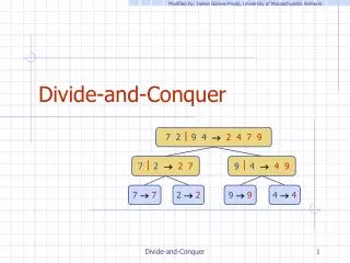
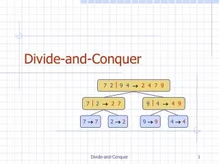
Mergesort • Split array A[0..n-1] in two about equal halves and make copies of each half in arrays B and C • Sort arrays B and C recursively • Merge sorted arrays B and C into array A
Mergesort Code mergesort( int a[], int left, int right) { if (right > left) { middle = left + (right - left)/2; mergesort(a, left, middle); mergesort(a, middle+1, right); merge(a, left, middle, right); } }
Analysis of Mergesort • T(N) = 2T(N/2) + N • All cases have same efficiency: Θ(n log n) • Space requirement: Θ(n) (not in-place) • Can be implemented without recursion (bottom-up)
Features of Mergesort All cases: Θ(n log n) Requires additional memory Θ(n) Recursive Not stable (does not preserve previous sorting) Never used for sorting in main memory, used for external sorting
Quicksort Let S be the set of N elements Quicksort(S): If N = 0 or N = 1, return Pick an element v - pivot, in S Partition S - {v} into two disjoint sets: S1 = {x є S - {v}| x ≤ v}, and S2 = {x є S - {v}| x ≥ v} Return {quicksort(S1), followed by v, followed by quicksort(S2)}
Quicksort • Select a pivot (partitioning element) • Median of three algorithm • Take the first, the last and the middle elements and sort them (within their positions). • Choose the median of these three elements. Hide the pivot – swap the pivot and the next to the last element. • Example: 5 8 9 14 2 7 After sorting 1 8 9 54 2 7 Hide the pivot 1 8 9 24 57
Quicksort Rearrange the list so that all the elements in the first s positions are smaller than or equal to the pivot and all the elements in the remaining n-s-1 positions are larger than or equal to the pivot. Note: the pivot does not participate in rearranging the elements. Exchange the pivot with the first element in the second subarray — the pivot is now in its final position Sort the two subarrays recursively
left – the smallest valid index right – the largest valid index if( left + 10 <= right) { int i = left, j = right - 1; for ( ; ; ) { while (a[++i] < pivot) {} while (pivot < a[--j] ) {} if (i < j) swap (a[i],a[j]); else break; } swap (a[i], a[right-1]); quicksort ( a, left, i-1); quicksort (a, i+1, right); } else insertionsort (a, left, right);
Analysis of Quicksort • Best case: split in the middle — Θ(n log n) T(N) = 2T(N/2) + N • Worst case: sorted array — Θ(n2) T(N) = T(N-1) + N • Average case: random arrays — Θ(n log n) Quicksort is considered the method of choice for internal sorting of large files (n ≥ 10000)
Features of Quicksort Best and average case: Θ(n log n) , Worst case: Θ(n2), it happens when the pivot is the smallest of the largest element In-place sorting, additional memory only for swapping Recursive Not stable Never used for life-critical and mission-critical applications, unless you assume the worst-case response time
Binary Search • Very efficient algorithm for searching in sorted array: K vs A[0] . . . A[m] . . . A[n-1] • If K = A[m], stop (successful search); • otherwise, continue searching by the same method in A[0..m-1] if K < A[m], and in A[m+1..n-1] if K > A[m]
Analysis of Binary Search • Time efficiency T(N) = T(N/2) + 1 • Worst case: O(log(n)) • Best case: O(1) • Optimal for searching a sorted array • Limitations: must be a sorted array (not linked list)
Binary Tree Algorithms • Binary tree is a divide-and-conquer ready structure Ex. 1: Classic traversals (preorder, inorder, postorder) • Algorithm Inorder(T) if T Inorder(Tleft) print(root of T) Inorder(Tright) • Efficiency: Θ(n)
Binary Tree Algorithms Ex. 2: Computing the height of a binary tree h(T) = max{ h(TL), h(TR) } + 1 if T and h() = -1 Efficiency: Θ(n)