Approximating the area under a curve using Riemann Sums
760 likes | 1.93k Vues
Approximating the area under a curve using Riemann Sums. Riemann Sums -Left, Right, Midpoint, Trapezoid Summations Definite Integration. We want to think about the region contained by a function, the x-axis, and two vertical lines x=a and x=b. . a. b.

Approximating the area under a curve using Riemann Sums
E N D
Presentation Transcript
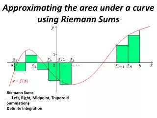
Approximating the area under a curve using Riemann Sums Riemann Sums -Left, Right, Midpoint, Trapezoid Summations Definite Integration
We want to think about the region contained by a function, the x-axis, and two vertical lines x=a and x=b. a b The goal of this process is to determine the area that is shaded yellow. We will first use geometry and some basic shapes to estimate the area. We will then combine the idea of limits with that of integrals to find the exact area.
There are two methods that we can use to approximate area. One is creating basic geometry figures and looking at each individual figure, finding its area, and then summing those values. This is not difficult if the number (n) of figures is small. • If n becomes very large (probably over 10) then this process can become very tedious and we revert to the idea of using summations and creating a ‘sigma notation formula’ that helps evaluate sums when n is large.
Since we know we will be using rectangles, and we know the formula for the area of a rectangle, we will start with the most basic style of problem. • When we look at the region under the curve, it will be bounded by two vertical lines and the x axis, in order to find the size of the intervals for a desired number of rectangles we will use this formula :
The area of each rectangle will then be the product of the height and width of that rectangle or subinterval. Then we will add up all “n” rectangles. • What do we use as the height of each rectangle? (later on we will learn that as more and more rectangles are made, this distinction does not matter) but for computational reasons we will talk about 4 methods • Right Sums (using right endpoints, right shoulder of rectangle touches the curve) • Left Sums (using left endpoints, left should of rectangle touches the curve) • Midpoint Sums (using the midpoints of each subinterval, so the segment containing the midpoint of the subinterval is used as the height for that rectangle. • Trapezoid (instead of using rectangles, a better approximation can be made using irregular trapezoids)
A few pictures to make the connection We want to divide it into “n” intervals, for this example let n = 6. So to determine how wide each interval is, we would take (b-a)/n, and that value is ∆x. Then to find the endpoint of the first interval you simply add a+∆x, then keep adding ∆x to the previous endpoint to get the next subinterval’s endpoint until you are done. Now we’ve simply constructed each rectangle so that each of the six rectangles are touching the curve with their right shoulders. Right shoulder of rectangle on curve, so right sum
The area of the second rectangle is A=height*width So, R2= f(x)*∆x You will then do this for each rectangle. Note to find f(x)’s numerical value you simply take the x value of that right endpoint of the rectangle and plug it into f(x) to find the actual numerical height of that rectangle. f(x)
Because all the rectangles go above f(x), the sum of the areas will be larger than the actual area under the curve, so if f(x) is increasing this is an overestimate. • Any ideas on how to make the green areas smaller?
Left Sum (puts left shoulder on f(x)) Left Shoulder is on the curve, Left Sum
Find the area of the rectangles in the same fashion as we did with right sums. The blue areas are under the curve, but are not included in your rectangle areas, so if f(x) is increasing the left sum would be an underestimate
Right Sum Left Sum By the sandwich theorem or squeeze theorem we know that since the Right sum is an overestimate, and the left sum is an underestimate, then the actual area under the curve is stuck somewhere in between them. Remember that the right sum will reduce down towards the actual area if we increase the number of rectangles, likewise the left sum will increase towards the actual area when we increase n because f(x ) is increasing in this graph.
Our goal is to eventually get the ∆x to be infinitely small, so that the overestimate or underestimate is infinitely small. So if we use the idea of limits then we can approach the actual area under the curve. That is as n approaches infinity we will get an exact value for the area.
Examples: Find the area under the curve Using 5 rectangles Then the first “right endpoint” is a+∆x
Find the area under the curve using 10 rectangles. Right Sum
Use Riemann Sums – Right Hand & Left Hand • n=5 [1,4]
Use Riemann Sums – Right Hand & Left Hand • 5 rectangles [-1.2,2]
Use Riemann Sums – Midpoint • 5 rectangles
Use Riemann Sums – Midpoint • 6 rectangles [6,12]
When the value of “n” is increased, the number of rectangles increases, does the right sum and left sum squeeze down towards the actual area? • Which is a better approximation
Find the area under the curve with n=6,12 Left and Right Sums
Using Midpoints gives a bit of a better approximation. • Steps • Still divide everything up into subintervals. • Locate the midpoints of each interval (endpoint + endpoint/2) • Now use the midpoint as the x value that you plug into f(x) to find the height of the rectangle. • Then to find the area of each rectangle you still take the height*∆x • Sum all rectangle areas.
This picture describes the concept of finding the heights of each rectangle at the midpoints of each subinterval. Still broke the interval into congruent sections, but then found the midpoints of those sections, plug that midpoint into f(x) to find the height of the rectangle. Notice how in each rectangle, the part of the rectangle above the curve is almost equivalent to the part of the rectangle not calculated under the curve, so the overestimate and underestimate almost cancel each other out completely
Use midpoints with a=1 and b=3 and n=10. The exact area is 21.20014476021 Is the midpoint method along with several subintervals very close to this value?
Use midpoints, left s um, and right sum. Which is a better estimate? f(x)=sin(x) , [0, pi] use 8 rectangles.
Trapezoids Notice after creating trapezoids, the area above or below the curve that is over or under estimated has become so small that coloring it in would be too difficult to do, this is a very good approximation, but the method is more involved and the steps are longer because of the formula for finding area of a trapezoid being more complex than the area of a rectangle.
The area of the curve using the trapezoid method is identical to the average of the left and right Riemann Sums.
Trapezoids give even better approximations. Remember the formula for finding a trapezoid is 1/2h*(b1+b2) Examples: Find the area under the curve using trapezoids.
USE Trapezoids. Which is a better estimate? f(x)=sin(x) , [0, pi] use 8 subintervals.
Riemann Sums when the number of rectangles or subintervals is very large. Height of the “ith” rectangle Width of the “ith” rectangle Counting tool that allows us to move from the 1strectangle to the 2nd rectangle to the 3rd … to the ith rectangle
Counting tool that allows us to move from the 1strectangle to the 2nd rectangle to the 3rd … to the ith rectangle This is for right sums. xi changes when dealing with left sums or with midpoints. If we are interested in going between a=1 and b=3 for example with n rectangles. Δx = (3-1)/n = 2/n 2nd 1st 3rd ith ith 4th ith 1 3 1+(2/n) 1+(2/n)i . . . 1+(2/n)3 1+(2/n)4 1+(2/n)2 f( ) will be the height of the ith rectangles.
So now lets look at the function Now in order to evaluate this you need to identify compute f(1+2i/n) so plug that in for every x in x2-x+1
Now simplify the expression and apply your limit rules to see what the limit approaches and that will be the area under the curve between a=1 and b=3.
Combining Riemann Sums with Summation Notation We will want to useias a counting device to move from one rectangle to the next.
Right Sum The ∆xi will put us at the right side of the beginning rectangle • Left Sum The ∆x(i-1) will put us at the left side of the beginning rectangle
Take the previous function, graph it, find the area using right sums when n=4. • Now take the previous slide’s expression and plug in 4 for n. • What do you notice? • This should always be the case… What happens when n=100000? What about n=10000000000?
Do you see how this allows us to bring in the idea of limits and allowing n to go to infinity, with the summation notation we will get the exact area if n approaches infinity.
Lets use the same function and compute the left sum. • The following function is using midpoints.
Complete this using the idea of Riemann sums and the summation formulas. What does the area go towards when n gets larger? 56.6666
We could do the same thing with left hand sums but as n get really large both the right hand sum and the left hand sum will converge to the same value. • Know that when f(x) is increasing on I the right sum will be an overestimate and the left sum will be an underestimate when n is small. • When f(x) is decreasing on I the right sum will an underestimate and the left sum will be on overestimate. • But the more and more rectangles we create the better approximations we get, and when n∞ we get an exact value for the area.
The idea of using summations and the corresponding formulas for i, can be very tedious with just the basic functions we have used so far, the algebra gets even more complicated when you raise something to a higher power or take the square root, it can all still be done using the summation formulas but we have more efficient methods. But it must be understood that these new methods all arose from the foundation of these summation formulas. The more efficient way is called definite integration.