Air Quality Modelling
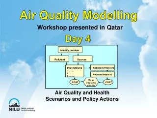
Air Quality Modelling. Workshop presented in Qatar. Day 3 Model application. Air Quality modelling -applications. Different models – different applications. Single source permits Urban assessments Future impacts Forecasts Mitigation options Compliance Public information

Air Quality Modelling
E N D
Presentation Transcript
Air Quality Modelling Workshoppresented in Qatar Day 3Model application
Air Quality modelling -applications Differentmodels – differentapplications • Single sourcepermits • Urban assessments • Futureimpacts • Forecasts • Mitigationoptions • Compliance • Public information • Policy decicions
C M Several types of models • Gaussian models • most used models for estimates of dispersion from stacks. • available for area sources and urban areas. • Box models • based upon budgets analysis • used in simple urban air pollution modelling. • Statistical models • based upon established relationships. • can not be used for planning purposes. • Numerical models • based upon numerical solutions of the continuity equations. • Several models have been developed and applied. • Trajectory / puff models • based upon knowledge of the wind field and the variations of winds • suited for dispersion from single sources at larger distances or in cases with space and time variations in meteorology
For single sources - stackemissions : The Gaussian plume model
The Gaussian plume models • Gaussianmodelssimplifytheturbulence to be spatiallyhomogenous (i.e. K=constant) and the wind speed to be constant with height • Efficient and effectivetools for calculatingplumedispersion from pointsources • Less applicablewithcomplexterrain, lowwind speeds or complexboundarylayerstructure • 3 basic types • Steady stateplumemodel • Segmentedplumemodel • Puff-trajectory type models
[ ] ( ) ( ( ) / u = - s × - s ps s 2 2 2 2 × C Q exp H / 2 y / 2 z y y z s = s = P q ax and bx y z Gaussian type dispersion models ) • where Q = release rate (µg/s) • H = effective plume height • = dispersion parameters (m) Source and surface specifications Coeff Unst. Neutr. Sl. Stable Stable Surface a 0.31 0.22 0.24 0.27 emission p 0.89 0.80 0.69 0.59 Low stacks b 0.07 0.10 0.22 0.26 Smooth surf q 1.02 0.80 0.61 0.50
Concentration at ground level along the wind direction
Gaussian plume models • Used for: • Permits. Assessimpact from plannedactions • Evaluateneededstackheights to meet AQ limit values • Estimatefuturecontributions from planned single sources
Power plant planning • Stack height : 14 m • Stack diameter: 2.74 m • Exit velocity 48 m/s • Exit gas temperature: 475 deg K • Vol flow 281 m3/s • NOx as NO2 emissions 18.4 kg/h = 5.1 g/s 2010
Future impact Estimatedgroundlevelconcentrationsof NO2 Max NO2: 28 µg/m3 = 14 % of AQ limit 1-3 km from power plant At 10 km away NO2 is l.t. 10 µg/m3
Puff-trajectory models For instationarymeteorologicalconditions • Puffs arereleased, e.g. every300 seconds, witha time stept • Theyare given an initial size and heightabovethestack, dependent on exit velocity, emissiontemperature, stability, wind speed and physicalstacksize • Puffs areadvectedeach time steptusingthewindvelocity from thenearest grid point • x = x0 + U t and y = y0 + V t • At the end of the hour their size is calculated σz(t) and σy(t)
Puff Trajectory Model “INPUF” Puffs are transported by the everchanging wind
Puffs as seen from the side Mixing height (MH) Puffs become well mixed if 0.8 σz > MH Puffs are combined if x < σz x H Stack Puffs are reflected at the surface
Puffs as seen from above Hour 1 Source Hour 3 Hour 2
The numerical dispersion model EPISODE • Meteorological hourly gridded input data: • Windfield (u, v, w) • Temperature at ground level • Vertical temperature gradient (stability) • Mixing height • Turbulence (v and w) Windfield Oslo - 1 km grid
Brickfactoryemissions Gabtali area: 108 brickkilns (stacks) Fuel: Mainlycoal (somewood) Consumption: about 4 tons/day Production: ~ 22 000 bricks/day Sulphurcontent: 3-4 % S ? Ashcontent: ??? Stackheight: 45 m Outletstack diametre: ~ 1 m Exit gas temperature: ? Wind rose Dhakawinter
Maximumgroundlevel concentrationsof SO2
Estimated 24-h concentration SO2 Aricha road Gabtali 33 stacks random positioned Lalmatia Kalabagan
Exercise #7: Concentrations from example stack using CONCX Estimatethemaximumconcentrationsof SO2 from thestack. Createnewstackcharacterstics and wind speeds basedontheexampleabove, and wewillcompareresults. What is themaxconc during unstableatmosphericconditions? What is thegroundlevelconc at ”x” km distance during neutralconditions?
Verifying compliance • LV/S/G related to: • Compound • Type of impact • Concentration • Averaging time • Local conditions • Compliance with: • Limit values • Standards • Guidelines
Guidelines Standards • Provide basis for protecting public health • Background information • Not intended to be standards Guidelines: Scientific basis Standards: Level of AQ adopted by regulatory authorities Enforceable Political choices Concentration + Averaging time
American Thoracic Society. What constitutes and adverse health effect of air pollution? American Journal of Respiratory and Critical Care Medicine, 2000, 161:665–673.
Health endpoints used in Burden of Disease assessment (2012) • Ambient particulate matter (PM): • Lower respiratory infections • Trachea, brunchus, and lung cancer • IHD • Cerebrovascular disease • COPD • Household air pollution (solid fuel) • As above; cataracts • Ambient ozone pollution • COPD • Source: Lim et al, Lancet 2012
Air Quality standard for PM10 (24 h average) (µg/m3) EU WHO France Taiwan USA Mauritius Mexico Brazil Malaysia Hong Kong Saudi Arabia Kuwait 0 50 100 150 200 250 300 350 400 Qatar
Verifying compliance Meeting standards and limit values • Monitoring • Modelling • Assessment % of urban populationpotentiallyexposed to air qualityexceeding standards
Exercise #8: AQ Standards Discussion • Whatinformation is necessary for theprocessof setting AQ standards? • Whatlocal (environmental) conditionsneed to be consideredwhen setting standards? • Whathealth and socialissuesneed to be considered? • For verification: howcanthis be done? • Shouldthere be changes/updates to the Qatar standards?
Emissions Meteorology Air Quality Model test and verification model test verification Operational dispersion model
Policy decisions and support EstimatedNOxconcentrations, HCMC NOx (µg/m3 )
Relative contribution Pre 2004 Future (2010?) AnnualaverageNOxconcentration
Exposure assessment Links population data to concentration fields Number of people exposed above the limit value of PM10 Oslo
For assessingcompliance All sources needed Other input data: Source data (stacks, lines , areas) Meteorology (winds, dispersion) Measurements (ifavailable) Measured 2-week average concentrationsof SO2 Wind rose Dhaka February 2013
Grid: 25 x 55 km PM10concentrations
Estimated PM10 conc. over Dhaka > 300 µg/m3 Bricksources included Compared to 24 h aver. limits: Bangladesh: 150 µg/m3 WHO : 50 µg/m3 PM10exceededdue to thesesourcesalone (brickkilns!)
Estimated SO2conc. over Dhaka WHO Guidelines 24 h aver: 20 µg/m3 Exceeded
Secondarypollutants - ozoneformation Numerical model domain Model top open boundary Western open boundary Boundaryconditions Eastern open boundary The open boundaries of the model domain. Estimates of the background concentration levels on these boundaries must be given as input data.
Regional model Modelling ozone concentrations • Total domain size of 100 km x 100 km • Horizontal grid spacing 5 km • 25 layers with increasing thickness upwards from the ground to a total height of 4 km above sea level Nested grid Combined global and localemission data
Input data Wind fieldcomputedwith TAPM Trafficemissions + all othersources….
Estimated ozone concentrations Largerscaleestimatedconcentrations used as boundaryconditions for detailed grid
Exampleestimateusing NILU models Sources at 25.89 degN 51.54 deg E Wind data august (TAPM) Stack data Hs = 100 m Q = 100 kg/h (28 g/s) W = 15 m/s Tg= 400 K Diam = 2 m
TAPM model Hourlymaxconcentration August Hourly maxconc 18 µg/m3
TAPM model Monthlyaverageconcentrations Wind rose 30 km
AirQUISEmissions/ DispersionExercise (Qatar Point Source) • Establishmeteorology (August 2011) • Wind speed • Wind direction • Net radiation • Establish GIS • Grid • Boundaries • Regions • Sources • EstablishLookups • Components • Units • Fuels • SourceSectors • Time variations • Enter source data • Industry/Stack Data • Process Data • Emissionfactors