Download
1 / 35
380 likes | 587 Vues
Air Quality Modelling. Lecture-1. What does model means?. Models reflects a mathematical description of hypothesis conveying the behavior of some physical process or other. Not exact replica but contain some of nature’s essential elements.

E N D
Air Quality Modelling Lecture-1
What does model means? • Models reflects a mathematical description of hypothesis conveying the behavior of some physical process or other. • Not exact replica but contain some of nature’s essential elements.
When the process of problem reduction or solution involves transforming some idealized form of the real world situation into mathematical terms, it goes under generic name of mathematical modelling. “Mathematical modelling is an activity which requires rather more than the ability just to solve complex sets of equations difficult through this may be”. Mathematical modelling utilizes ANALOGY to help understand the behavior of complex system. What is mathematical modelling?
What is physical modelling? • In physical modelling nature is simulated on a smaller scale in the laboratory by a physical experiment. • When detailed mathematical models and/ or experimental field measurements become very costly, laboratory simulation using scaled down models in wind tunnels or water channels is often the best approach.
Concept of mathematical modelling applied to air pollution Mathematical Modelling Source Receptor Transport Source: Point, Line, Area. Receptors: Humans. Transport :Decides fate of air pollution Re-entertainment: Re suspension of air pollutants.
Air Quality Models Analogy - helps in explaining / understanding unfamiliar situations. Ex: Children playing father/ mother game Expectant mothers: practice nappy changing on dolls. Models: Not exact replica but contain some of nature’s essential elements. Ex: When expectant mother practice nappy changing to dolls, dolls are laying still while in reality, babies do not lie still!. Hence, models reflects a mathematical description of hypothesis conveying the behavior of some physical process or other.
What is air quality model A mathematical relationship between emissions and air quality that incorporates the transport, dispersion and transformation of compounds emitted into the air. System approach to air quality model
Models are not a unique representation as they never completely replicate a system. But models are useful tool in the design of new, large or otherwise modified existing processes or systems. Conventional method of designing physical models replicating a process or system is time consuming and cumbersome process. Physical models sometime can not replicate a system which is having complicated heat and mass transfer processes. Mathematical models therefore is able to cope reasonably well with such processes or systems provided each is built into the set of mathematical equations. Model objective
Model categories Broad Categories Steady state models Dynamic models Discreet system modelling Empirical model Continuous system modelling Suggested readings: M. Crossal A.O. Moscardini, “Learning art of mathematical modelling”, Ellis Harmood Publication
Air Quality Models STATISTICAL DETERMINISTIC PHYSICAL REGRESSION EMPIRICAL WINDTUNNEL SIMULATION STEADY STATE TIME DEPENDENT GAUSSIAN PLUME SPECTRAL BOX GRID PUFF TRAJECTORY EULERIAN LAGRANGIAN Suggested readings: Weber, E., “Air pollution assessment modelling methodology”, NATO, challenges of modern society, vol.2, Plenum press, 1982
What is deterministic approach? The deterministic mathematical models calculate the pollutant concentrations from emission inventory and meteorological variables according to the solution of various equations that represent the relevant physical processes. Deterministic modelling is the traditional approach for the prediction of air pollutant concentrations in urban areas.
Deterministic approach: Basics • What is Transport: • It is also termed as advection • Most obvious effect of atmosphere on emission • Advection: implies transport of pollutant downwind of source • What is Dilution? • It is also termed as “mixing”. • It is accomplished through “turbulence” • Mainly atmospheric turbulence is active • What is Dispersion? • Dispersion = Advection (Transport) + Dilution = Advection +Diffusion or
Basic mathematical equation where C = pollutant concentration; t = time; = wind vector; Q = source term; R = removal term ; = turbulent flux of pollutants
Deterministic based AQM The deterministic based air quality model is developed by relating the rate of change of pollutant concentration in terms of average wind and turbulent diffusion which, in turn, is derived from the mass conservation principle. where C = pollutant concentration; t = time; x, y, z = position of the receptor relative to the source; u, v, w =wind speed coordinate in x, y and z direction; Kx, Ky, Kz = coefficients of turbulent diffusion in x, y and z direction; Q = source strength; R = sink (changes caused by chemical reaction). The above diffusion equation is derived in several ways under different set of assumptions for development of air quality models Gaussian model is one of the mostly used air quality model based on ‘deterministic principle’ Reference: Cheremisinoff, P.N.,1989. Encyclopedia of environmental control technology: air pollution control. Volume 2, Gulf Publishing Company, Houston.
Gaussian plume Dispersion model: Assumptions • Steady-state conditions, which imply that the rate of emission from the point source is constant. • Homogeneous flow, which implies that the wind speed is constant both in time and with height (wind direction shear is not considered). • Pollutant is conservative and no gravity fallout. • Perfect reflection of the plume at the underlying surface, i.e. no ground absorption. • The turbulent diffusion in the x-direction is neglected relative to advection in the transport direction , which implies that the model should be applied for average wind speeds of more than 1 m/s (> 1 m/s). • The coordinate system is directed with its x-axis into the direction of the flow, and the v (lateral) and w (vertical) components of the time averaged wind vector are set to zero. • The terrain underlying the plume is flat • All variables are ensemble averaged, which implies long-term averaging with stationary conditions.
Gaussian Plume Dispersion Model Where C : concentration of emission (gm/m3) at any receptor location at x (downwind distance from source), y (crosswind), and z (vertical) Q : source emission rate (gm/sec) u : horizontal wind velocity He : plume centre line height above ground z : vertical standard deviation of emission distribution y : horizontal standard deviation of emission distribution
Application: Gaussian Based Vehicular Pollutant Dispersion Model The basic approach for development of deterministic vehicular pollution (line source) model is the coordinate transformation between wind coordinate system (X1, Y1, Z1) and line source coordinate system (X, Y, Z). A hypothetical line source is assumed to exist along Y1 that makes the wind direction perpendicular to it (Figure 1). The concentration at receptor is given by Csanady (1972): Reference: Csanday, G.T., 1972. Crosswind shear effects on atmospheric diffusion. Atmospheric Environment, 6,221-232.
Numerical approach Numerical models also comes under deterministic modelling technique which are based on numerical approximation of partial differential equations representing atmospheric dispersion phenomena. Basic mathematical equation The term Ft in the above equation is unknown and diffused equation is not in close form. Reference: Juda, K., 1986. Modelling of the air pollution in the Cracow area. Atmospheric Environment, 20 (12), 2449-2458.
Basis for numerical approach First order closure models, also called K- models, have their common roots in the atmospheric diffusion equation derived by using a K-theory approximation for the closure of the turbulent diffusion equation. The first order closure models are time dependent. Numerical based AQM Eulerian grid model (Danard, M.B., 1972) Lagrangian trajectory model (Johnson, 1981) Hybrid of eulerian-lagrangian model (Particle-in-cell) (Sklarew et al., 1972) Random walk (Monte-Carlo) trajectory particle model (Joynt and Blackman, 1976) Mostly used numerical based AQM Gaussian puff model (Hanna et al., 1982) Reference: Danard, M.B., 1972. Numerical modelling of carbon monoxide concentration near a Highway. Journal of Applied Meteorology, 11, 947-957. Johnson, W.B., 1981. Interregional exchanges of air pollution: model types and application. In Air pollution modelling and its application-I, Edited by Wispelaere, C. De., Plenum Press, New York. Sklarew, R.C., Fabrick, A.J. and Prager, J.E., 1972. Mathematical modelling of photochemical smog the using PIC method. Journal of Air Pollution Control Association, 22, 865-. Joynt, R.C. and Blackman, D.R., 1976. A numerical model of pollutant transport. Atmospheric Environment, 10, 433-. Hanna, S.R., Brigs, G.A. and Hosker, Jr. R.P., 1982. Handbook on atmospheric diffusion. National Technical Information Centre, U.S. Department of Energy, Virginia.
STATISTICAL APPROACH Statistical models calculate pollutant concentrations by statistical methods from meteorological and emission parameters after an appropriate statistical relationship has been obtained empirically from measured concentration Basis for statistical approach Regression and multiple regression models (Comrie, 1997) Regression models describes the relationship between predictors (meteorological and emission parameters) and predictant (pollutant concentrations) Time series models (Box and Jenkins, 1976) Time series analysis is purely based on statistical method applicable to non repeatable experiments. Box-Jenkins approach extracts all the trends and serial correlations among the air quality data until only a sequence of white noise (shock) remains. The extraction is accomplished via the difference, autoregressive and moving average operators. Reference: Comrie, A. C., 1997. Comparing neural networks and regression model for ozone forecasting. Journal of Air and Waste Management Association, 47, 653-663 Box, G.E.P. and Jenkins, G.M., 1976. Time series analysis forecasting and control. 2nd Edition, Holdenday, San Francisco.
Basic mathematical equation The Box –Jenkins (B-J) models are empirical models created from the historical data. Statistical graphs of the autocorrelation function (ACF) and partial autocorrelation function (PACF) to identify an appropriate time series model. The general class of univariate B-J seasonal models, denoted by ARIMA (p, d, q)(P, D, Q)s can be expressed as: Where and = regular and seasonal autoregressive parameters, B = backward shift operators, =difference operators, d and D = order of regular and seasonal differencing, s= period/span, zt = observed data series, and Θ = regular and seasonal moving average parameters, at = random noise, p, P, q and Q represent the order of the model and c = constant.
Mostly used stochastic based AQM Time series model Univariate model Multivariate model Bivariate model - 24 h avg.. CO model with wind speed as input - 24 h avg.. CO model with temperature as input - Max. daily 1-h avg.. CO model with wind speed as input - Max. daily 1-h avg.. CO model with temperature as input - Max. daily working hours 1-hour avg.. CO model with wind speed as input - Max. daily working hours 1-hour avg.. CO model with temperature as input - Hourly average CO model with wind speed as input - Hourly average CO model with temperature as input - 24 h avg.. CO model - Max. daily 1-h avg.. CO model - Max. daily working hours (8 AM - 8PM) 1-hour CO model - Hourly average CO model - 24 h avg.. CO model with temperature and wind speed as inputs - Max. daily 1-h avg.. CO model with wind speed and temperature as inputs - Max. daily working hours 1-hour avg.. CO model with wind speed and temperature as inputs Reference: Khare, M. and Sharma, P., 2002. Modelling urban vehicle emissions. WIT press, Southampton, UK. Sharma, P. and Khare, M., 2001. Short-time, real – time prediction of extreme ambient carbon monoxide concentrations due to vehicular exhaust emissions using transfer function noise models. Transportation Research D6, 141-146.
Double walled panel with thermocole Toughned glass panel 2.0m Ø1.8m 2.0m Cross section of the panel of test Turntable in panel no. 2 at test section floor section Air in Power section 6.0m Transition section Diffuser Test section Contraction cone 3.0m 3.0m 5.0m 6 7 8 1 3 4 5 0.6m 3.0m 2.5m 3.5m 0.6m 8 panels of 2m each = 16m 2.5m 0.8m Heating arrangement Turntable Speed control unit Door with handle Layout of environmental wind tunnel ENVIRONMENTAL WIND TUNNEL- IIT DELHI Physical modelling approach – Wind Tunnel • 26 m long, suction type, low wind speed, 16 m test section, 8 panels, 2 m each • EWT consists of entrance section, honeycomb section, wire mesh screen filters, test section, exit contraction section, transition and diffuser section • Turntable of 1.8 m diameter • Plenum chamber for prevention of surge and other disturbances, 6 m x 5 m wall
Basis for physical approach • The physical simulation studies using wind tunnels have shown high potential to understand complex urban dispersion phenomenon. • The pollutant concentrations measured within the physical model can be converted to equivalent atmospheric concentrations through the use of appropriate scaling relationship. • In the physical simulation studies of exhaust dispersion, the model vehicle movement system (MVMS) plays a vital role. The vehicle-induced turbulence can be understood accurately by using MVMS. Design consideration for MVMS* • maintenance of ‘‘no slip’’ boundary condition in atmospheric boundary layer (ABL) flow, • variations in traffic volume and traffic speed for two-way traffic, • operation of MVMS for various street configurations, • variation in approaching wind directions and wind speed, • operation of vehicles in different lanes. Reference: *Ahmad, K., Khare, M. and Chaudhry, K.K. 2005. Wind tunnel simulation studies on dispersion at urban street canyons and intersections- a review. Journal of Wind Engineering and Industrial Aerodynamics, 93, 697-71 Eskridge, R.E. and Hunt, J.C.R., 1979. Highway modelling-I: prediction of velocity and turbulence fields in the wake of vehicles. Journal of Applied Meteorology, 18 (4), 387- 400.
Plan of MVMS for urban street DESIGNED IN ENVIRONMENTAL WIND TUNNEL- IIT DELHI
PLAN OF MVMS FOR URBAN INTERSECTION DESIGNED IN ENVIRONMENTAL WIND TUNNEL- IIT DELHI
Wind tunnel based AQM • Development, testing and validation of atmospheric dispersion models through EWT generated database in a variety of atmospheric conditions. • Systematic understanding of the pollutants dispersion characteristics for line source (automobile exhaust emissions), point source (stack emissions) and area source (low level areal emissions) in plain and complex terrains, such as, hills and valleys. • Understanding of the dispersive behavior of toxic gases from accidental releases. • Studies on the effects of pollutants on plants and buildings under dynamic environmental conditions for various geographical conditions. • Simulation of ‘heat islands’ and its effect on pollutant dispersion. • Location of ‘hot spots’ at the urban intersections. Reference: Eskridge, P.E. and Thompson, R.S., 1982. Experimental and theoretical study of the wake of a block-shaped vehicle in a shear-free boundary flow. Atmospheric Environment, 16 (12), 2821-2836. Snyder, W.H., 1972. Fluid models for the study of air pollution meteorology: similarity facilities, review of literature and recommendations, U.S. Environmental Protection Agency, Washington.
LIMITATIONS OF MODELS Deterministic models: • Inadequate dispersion parameters • Inadequate treatment of dispersion upwind of the road • Requires a cumbersome numerical integration especially when the wind forms a small angle with the roadways. • Gaussian based plume models perform poorly when wind speeds are less than 1m/s. • Numerical models have common limitations arising from employing the K-theory for the closure of diffusion equation. The K-theory diffusion equation is valid only if the size of the ‘plume’ or ‘puff’ of pollutants is greater than the size of the dominant turbulent eddies. • The Gaussian puff model relative diffusion parameters are derived from very few field experiments, which limits its applicability. • The other limitations of numerical models are large computational costs in terms of time and storage of data. It also requires large amounts of input data.
LIMITATIONS OF MODELS Statistical models: • Require long historical data sets and lack of physical interpretation. • Regression modelling often underperforms when used to model non-linear systems. • Time series modelling requires considerable knowledge in time series statistics i.e. autocorrelation function (ACF) and partial auto correlation function (PACF) to identify an appropriate air quality model. • Statistical models are site specific. • Hybrid model prediction accuracy depends on the selection of suitable deterministic model and identification of appropriate statistical distribution parameter. • Application of hybrid approach to strongly auto correlated and/or non-stationary data requires specific treatment for auto correlation /non stationary to increase prediction accuracy.
LIMITATIONS OF MODELS • In ANN based vehicular pollution model, the main problem facing when training neural network model, is deciding upon the network architecture (i.e., number of hidden layers, number of nodes in hidden layers and their interconnection). • At present, no procedures has been established for selecting proper network architecture, rather than training several network architecture and choose the best out of them. • Multilayer neural network performs well when used for interpolation, but poorly, if used for extrapolation. • No thumb rules exist in selection of data set for training, testing and validation of neural network based model.
LIMITATIONS OF MODELS* Physical models: wind tunnel • The major limitations of wind tunnel studies are construction and operational cost. • Simulation of real time air pollution dispersion is expensive. • Real time forecast is not possible. *Reference: Juda, K., 1989. Air pollution modelling. In: Cheremisinoff, P.N. (Eds.), Encyclopedia of Environmental Control Technology, Vol. 2: Air Pollution Control, Gulf Publishing Company, Houston, Texas, USA, pp.83-134. Nagendra, S.M.S. and Khare, M., 2002. Line source emission modelling- review. Atmospheric Environment, 36 (13), 2083-2098.
Application : Area source Principle : (i) It assumes uniform mixing throughout the volume of a three dimensional box. (ii) Steady state emission and atmospheric conditions. (iii) No upwind background concentration. - Model description where C = steady state concentration x = distance over which the emission takes place qa = Area emission rate L = mixing height u = mean wind speed through vertical extent box Box Model C = x qa / (Lu)
Box model u L C = uniform qa x Suggested reading: Lyons, T.J. and Scott, W.D. “Principles of air pollution meteorology”, Behavan press, 1990
Application motor vehicle travelling along a straight section of highway OR agricultural burning along the edge of a field OR line of industrial sources on the bank of a river Assumption Infinite length source continuously emitting the pollution Ground level source Wind blowing perpendicular to the line source Line source model - Model: C (x) = (2q)/(2 z u) u Line source q = emission per unit of distance along the line (gm/m-sec) q (gm/sec) x Receptor
CONCLUSIONS • Air pollution in cities is a serious public health problem. Therefore, there is need for reliable air quality management system for abatement of urban air pollution problem. • Several air quality models have been developed using deterministic, statistical and physical approaches for urban air quality management. • These three modelling approaches have been used in the development and validation of vehicular pollution dispersion models pertaining to urban context in Delhi. • Limitations of deterministic modelling approach is assumptions considered in describing vehicular pollution dispersion phenomena. • Limitations of statistical modelling approach is selection of modelling parameters representing the appropriate statistical distribution of air quality data. • Limitations of physical modelling approach is high cost involvement in simulating real time vehicular pollution dispersion in laboratory.