Chapter 9 -- Simplification of Sequential Circuits
Chapter 9 -- Simplification of Sequential Circuits. Redundant States in Sequential Circuits. Removal of redundant states is important because Cost : the number of memory elements is directly related to the number of states

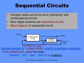
Chapter 9 -- Simplification of Sequential Circuits
E N D
Presentation Transcript
Redundant States in Sequential Circuits Removal of redundant states is important because • Cost: the number of memory elements is directly related to the number of states • Complexity: the more states the circuit contains, the more complex the design and implementation becomes • Aids failure analysis: diagnostic routines are often predicated on the assumption that no redundant states exist
Equivalent States • States S1, S2, …, Sj of a completely specified sequential circuit are said to be equivalent if and only if, for every possible input sequence, the same output sequence is produced by the circuit regardless of whether S1, S2, …, Sj is the initial state. • Let Si and Sj be states of a completely specified sequential circuit. Let Sk and Sl be the next states of Si and Sj, respectively for input Ip. Si and Sj are equivalent if and only if for every possible Ip the following are conditions are satisfied. • The outputs produced by Si and Sj are the same, • The next states Sk and Sl are equivalent.
Equivalent States Illustration Figure 9.1
Equivalence Relations • Equivalence relation: let R be a relation on a set S. R is an equivalence relation on S if and only if it is reflexive, symmetric, and transitive. An equivalence relation on a set partitions the set into disjoint equivalence classes. • Example: let S = {A,B,C,D,E,F,G,H} and R = {(A,A),(B,B),(B,H),(C,C),(D,D),(D,E),(E,E),(E,D),(F,F),(G,G),(H,H), (H,B)}. Then P = (A)(BH)(C)(DE)(F)(G) • Theorem: state equivalence in a sequential circuit is an equivalence relation on the set of states. • Theorem: the equivalence classes defined by the state equivalence of a sequential circuit can be used as the states in an equivalent circuit.
Methods for Finding Equivalent States • Inspection • Partitioning • Implication Tables
Finding Equivalent States By Inspection Figure 9.2
Finding Equivalent States by Partitioning Figure 9.3
Example 9.2 -- Partitioning example Figure 9.4
Example 9.3 -- Another partitioning example Figure 9.5
Example 9.5 -- Using implication tables to find equivalent states Figure 9.8
Incompletely Specified Circuits • Next states and/or outputs are not specified for all states • Applicable input sequences: an input sequence is applicable to state, Si, of an incompletely specified circuit if and only if when the circuit is in state Si and the input sequence is applied, all next states are specified except for possible the last input of the sequence. • Compatible states: two states Si and Sj are compatible if and only if for each input sequence applicable to both states the same output sequence will be produced when the outputs are specified. • Compatible states: two states Si and Sj are compatible if and only if the following conditions are satisfied for any possible input Ip • The outputs produced by Si and Sj are the same, when both are specified • The next states Sk and Sl are compatible, when both are specified. • Incompatible states: two states are said to be incompatible if they are not compatible.
Compatibility Relations • Compatibility relation: let R be a relation on a set S. R is a compatibility relation on S if and only if it is reflexive and symmetric. A compatibility relation on a set partitions the set into compatibility classes. They are typically not disjoint. • Example: let S = {A,B,C,D,E} and R = {A,A),(B,B),(C,C),(D,D),(E,E),(A,B),(B,A),(A,C),(C,A), (A,D), (D,A),(A,E),(E,A),(B,D),(D,B),(C,D),(D,C),(C,E),(E,C)} Then the compatibility classes are (AB)(AC)(AD)(AE)(BD)(CD)(CE)(ABD)(ACD)(ACE) The incompatibility classes are (BC)(BE)(DE) • Compatible pairs may be found using implication tables • Maximal compatibles may be found using merger diagrams
Examples 9.8 and 9.9 -- Generating Maximal Compatibles and Incompatibles
Merger diagrams Figure 9.11
Example 9.10 -- Merger diagrams for example 9.8 Figure 9.12
Minimization Procedure Select a set of compatibility classes so that the following conditions are satisfied • Completeness: all states of the original machine must be covered • Consistency: the chosen set of compatibility classes must be closed • Minimality: the smallest number of compatibility classes is used
Bounding the number of states • Let U be the upper bound on the number of states needed in the minimized circuit • Then U = minimum (NSMC, NSOC) • where NSMC = the number of sets of maximal compatibles • and NSOC = the number of states in the original circuit • Let L be the lower bound on the number of states needed in the minimized circuit • Then L = maximum(NSMI1, NSMI2,…, NSMIi) • where NSMIi = the number of states in the ith group of the set of maximal incompatibles of the original circuit.
State Reduction Algorithm • Step 1 -- find the maximal compatibles • Step 2 -- find the maximal incompatibles • Step 3 -- Find the upper and lower bounds on the number of states needed • Step 4 -- Find a set of compatibility classes that is complete, consistent, and minimal • Step 5 -- Produce the minimum state table
Example 9.11 -- Reduced state table corresponding to example 9.8 Figure 9.13
Example 9.12 -- State reduction problem Figure 9.14
Example 9.13 -- Another state table reduction problem Figure 9.15
Example 9.14 -- Yet another state reduction problem Figure 9.16
Example 9.15 -- Optimal state assignments Figure 9.17
Unique State Assignments for Four States Figure 9.18
State Assignments for a Four State Machine Figure 9.19
D flip-flop realization for assignment 1 Figure 9.20
D flip-flop realization for assignment 2 Figure 9.21
D flip-flop realization for assignment 3 Figure 9.22
State adjacencies for four-state assignments Assignment 1 Assignment 2 Assignment 3 Figure 9.23
Example 9.18 -- Implication Graphs Figure 9.24
Example 9.19 -- Closed subgraphs Figure 9.24
Example 9.20 -- Optimal state assignment Figure 9.26
Example 9.21 -- Another state assignment problem Figure 9.27
A D flip-flop realization of the previous example Figure 9.28
Example 9.24 -- Closed partitions Figure 9.29
Example 9.25 -- Cross dependency Figure 9.30