Lecture 20: Shortest Paths
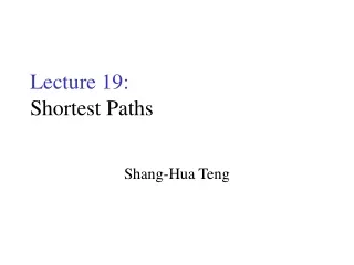
Lecture 20: Shortest Paths. Shang-Hua Teng. BOS. v. ORD. 4. JFK. v. v. 2. 6. SFO. DFW. LAX. v. 3. v. 1. MIA. v. 5. Weighted Directed Graphs. 2500. Weight on edges for distance. 1800. 800. 900. 1000. 400. Shortest Paths.

Lecture 20: Shortest Paths
E N D
Presentation Transcript
Lecture 20:Shortest Paths Shang-Hua Teng
BOS v ORD 4 JFK v v 2 6 SFO DFW LAX v 3 v 1 MIA v 5 Weighted Directed Graphs 2500 • Weight on edges for distance 1800 800 900 1000 400
Shortest Paths • Given a weighted, directed graph G=(V, E) with weight function w: ER. The weight of path p=<v0, v1,..., vk> is the sum of the weights of its edges: • We define the shortest-path weight from u to v by • A shortest path from vertex u to vertex v is any path with w(p)=(u, v) If there is a path from u to v, Otherwise.
Variants of Shortest Path Problem • Single-source shortest paths problem • Finds all the shortest path of vertices reachable from a single source vertex s • Single-destination shortest-path problem • By reversing the direction of each edge in the graph, we can reduce this problem to a single-source problem • Single-pair shortest-path problem • No algorithm for this problem are known that run asymptotically faster than the best single-source algorithm in the worst case • All-pairs shortest-path problem
Relaxation • For each vertex vV, we maintain an attribute d[v], which is an upper bound on the weight of a shortest path from source s to v. We call d[v] a shortest-path estimate. Possible Predecessor of v in the shortest path
Relaxation • Relaxing an edge (u, v) consists of testing whether we can improve the shortest path found so far by going through u and, if so, update d[v] and [v] By Triangle Inequality
Coping with Negative Weights • Deciding whether there is a negative circle • If the graph does not have a negative circle reachable from the source s, for the shortest path tree.
Initialize d[], which will converge to shortest-path value Relaxation: Make |V|-1 passes, relaxing each edge Test for solutionUnder what condition do we get a solution? Bellman-Ford Algorithm BellmanFord() for each v V d[v] = ; d[s] = 0; for i=1 to |V|-1 for each edge (u,v) E Relax(u,v, w(u,v)); for each edge (u,v) E if (d[v] > d[u] + w(u,v)) return “no solution”; Relax(u,v,w): if (d[v] > d[u]+w) then d[v]=d[u]+w
Bellman-Ford Algorithm What will be the running time? BellmanFord() for each v V d[v] = ; d[s] = 0; for i=1 to |V|-1 for each edge (u,v) E Relax(u,v, w(u,v)); for each edge (u,v) E if (d[v] > d[u] + w(u,v)) return “no solution”; Relax(u,v,w): if (d[v] > d[u]+w) then d[v]=d[u]+w
Bellman-Ford Algorithm What will be the running time? A: O(VE) BellmanFord() for each v V d[v] = ; d[s] = 0; for i=1 to |V|-1 for each edge (u,v) E Relax(u,v, w(u,v)); for each edge (u,v) E if (d[v] > d[u] + w(u,v)) return “no solution”; Relax(u,v,w): if (d[v] > d[u]+w) then d[v]=d[u]+w
Bellman-Ford Algorithm B BellmanFord() for each v V d[v] = ; d[s] = 0; for i=1 to |V|-1 for each edge (u,v) E Relax(u,v, w(u,v)); for each edge (u,v) E if (d[v] > d[u] + w(u,v)) return “no solution”; Relax(u,v,w): if (d[v] > d[u]+w) then d[v]=d[u]+w -1 s 2 A E 2 3 1 -3 4 C D 5 Ex: work on board
Bellman-Ford • Note that order in which edges are processed affects how quickly it converges • Correctness: show d[v] = (s,v) after |V|-1 passes • Lemma: d[v] (s,v) always • Initially true • Let v be first vertex for which d[v] < (s,v) • Let u be the vertex that caused d[v] to change: d[v] = d[u] + w(u,v) • Then d[v] < (s,v) (s,v) (s,u) + w(u,v) (Why?) (s,u) + w(u,v) d[u] + w(u,v) (Why?) • So d[v] < d[u] + w(u,v). Contradiction.
Bellman-Ford • Prove: after |V|-1 passes, all d values correct • Consider shortest path from s to v:s v1 v2 v3 v4 v • Initially, d[s] = 0 is correct, and doesn’t change (Why?) • After 1 pass through edges, d[v1] is correct (Why?) and doesn’t change • After 2 passes, d[v2] is correct and doesn’t change • … • Terminates in |V| - 1 passes: (Why?) • What if it doesn’t?
Properties of Shortest Paths • Triangle inequality • For any edge (u,v) in E, d(s,v) <= d(s,u) + w(u,v) • Upper bound property • d[v] >= d(s,v) • Monotonic property • d[v] never increase • No-path property • If v is not reachable then d[v] = d(s,v) = infty
Properties of Shortest Paths • Convergence property • If (u,v) is on the shortest path from s to v and if d[u] = d(s,u) at any time prior to relaxing (u,v), then d[v] = d(s,v) at all time afterward • Path-relaxation property • If p=< s=v0,v1, v2,..., vk> is the shortest path from s to vk and edges of p are relaxed in order in the index, then d[vk] = d(s, vk). This property holds regardless of any other relaxation steps that occur, even if they are intermixed with relaxations of the edges of p
Properties of Shortest Paths • Predecessor-subgraph property • Once d[v] = d(s,v), the predecessor subgraph is a shortest-paths tree rooted at s
Matrix Basic • Vector: array of numbers; unit vector • Inner product, outer product, norm • Matrix: rectangular table of numbers, square matrix; Matrix transpose • All zero matrix and all one matrix • Identity matrix • 0-1 matrix, Boolean matrix, matrix of graphs
Matrix Operations • Matrix-vector operation • System of linear equations • Eigenvalues and Eigenvectors • Matrix matrix operations