Lecture 19: Shortest Paths
230 likes | 250 Vues
Explore the concept of shortest paths in weighted, directed graphs, including variants of the shortest path problem, applications, algorithmic impacts, and more. Learn about Dijkstra's algorithm, optimal substructure, negative-weight edges, and algorithms like Breadth-First Search. Discover the properties and importance of shortest paths.

Lecture 19: Shortest Paths
E N D
Presentation Transcript
Lecture 19:Shortest Paths Shang-Hua Teng
BOS v ORD 4 JFK v v 2 6 SFO DFW LAX v 3 v 1 MIA v 5 Weighted Directed Graphs 2500 • Weight on edges for distance 1800 800 900 1000 400
Shortest Paths • Given a weighted, directed graph G=(V, E) with weight function w: ER. The weight of path p=<v0, v1,..., vk> is the sum of the weights of its edges: • We define the shortest-path weight from u to v by • A shortest path from vertex u to vertex v is any path with w(p)=(u, v) If there is a path from u to v, Otherwise.
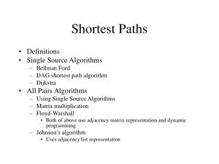
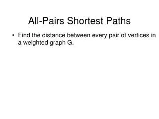
Variants of Shortest Path Problem • Single-source shortest paths problem • Finds all the shortest path of vertices reachable from a single source vertex s • Single-destination shortest-path problem • By reversing the direction of each edge in the graph, we can reduce this problem to a single-source problem • Single-pair shortest-path problem • No algorithm for this problem are known that run asymptotically faster than the best single-source algorithm in the worst case • All-pairs shortest-path problem
Applications of Shortest Path • Every where!!! • Driving (GPS) • Internet: network routing • Flying: Airline route • Resource allocation • VLSI design: wire routing • Computer Games • Mapquest, Yahoo map program
Optimal Substructure of Shortest-Paths • Lemma: (Subpath of shortest paths are shortest paths). • Let p=<v1, v2,..., vk> be a shortest path from vertex v1 to vk, and for any i and j such that 1 i j k, let pij = <v1i, v2,..., vj> be the sub-path of p from vertex vi to vj. Then pij is a shortest path from vertex vi to vj.
Algorithmic Impact • Greedy • Dynamic Programming
Negative-Weight Edges and Cycles • In general, edges might have negative weights • What if there is a negative-weight cycle • No shortest path can contain a negative cycle • Of course, a shortest path cannot contain a positive-weight cycle
Graph with Unit Weights • Special case: All weights are 1 • The single source shortest path problem can be solved by BFS • BFS tree explicit gives a shortest path from a source s to any vertex reachable from s
Breadth-First Search BFS(G, s) • For each vertex u in V – {s}, • color[u] = white; d[u] = infty; p[u] = NIL • color[s] = GRAY; d[s] = 0; p[s] = NIL; Q = {} • ENQUEUE(Q,s) // Q is a FIFO queue • while (Q not empty) • u = DEQUEUE(Q) • for each v Adj[u] • if color[v] = WHITE • then color[v] = GREY • d[v] = d[u] + 1; p[v] = u • ENQUEUE(Q, v); • color[u] = BLACK;
Breadth-first Search • Visited all vertices reachable from the root • A spanning tree • For any vertex at level i, the spanning tree path from s to i has i edges, and any other path from s to i has at leasti edges (shortest path property)
Breadth-First Search: the Color Scheme • White vertices have not been discovered • All vertices start out white • Grey vertices are discovered but not fully explored • They may be adjacent to white vertices • Black vertices are discovered and fully explored • They are adjacent only to black and gray vertices • Explore vertices by scanning adjacency list of grey vertices
Graphs with Non-Negative Weights • Shortest Path Tree • Can we use a similar idea to generate a shortest path tree which represents the shortest path from s to all vertices that are reachable from s?
Dijkstra’s Algorithm • Solve the single-source shortest-paths problem on a weighted, directed graph and all edge weights are nonnegative • Data structure • S: a set of vertices whose final shortest-path weights have already been determined • Q: a min-priority queue keyed by their d values • Idea • Repeatedly select the vertex uV-S (kept in Q) with the minimum shortest-path estimate, adds u to S, and relaxes all edges leaving u
BFS vs Dijkstra’s Algorithm BFS(G, s) | Dijkstra(G,s) • For each vertex u in V – {s}, • color[u] = white; d[u] = infty; p[u] = NIL • color[s] = GRAY; d[s] = 0; p[s] = NIL; Q = {} • ENQUEUE(Q,s) | ENQUEUE(Q,(s,d[s])) • while (Q not empty) • u = DEQUEUE(Q) | u = EXTRACT-MIN(Q) • for each v Adj[u] • if color[v] = WHITE | d[v] > d[u] + w(u,v) • then color[v] = GREY • d[v] = d[u] + 1; p[v] = u | d[v] = d[u] +w(u,v) • ENQUEUE(Q, v); | ENQUEUE(Q, (v,d[v])) • color[u] = BLACK;
Relaxation • For each vertex vV, we maintain an attribute d[v], which is an upper bound on the weight of a shortest path from source s to v. We call d[v] a shortest-path estimate. Possible Predecessor of v in the shortest path
Relaxation • Relaxing an edge (u, v) consists of testing whether we can improve the shortest path found so far by going through u and, if so, update d[v] and [v] By Triangle Inequality
Properties of Shortest Paths • Triangle inequality • For any edge (u,v) in E, d(s,v) <= d(s,u) + w(u,v) • Upper bound property • d[v] >= d(s,v) • Monotonic property • d[v] never increase • No-path property • If v is not reachable then d[v] = d(s,v) = infty
Properties of Shortest Paths • Convergence property • If (u,v) is on the shortest path from s to v and if d[u] = d(s,u) at any time prior to relaxing (u,v), then d[v] = d(s,v) at all time afterward • Path-relaxation property • If p=< s=v0,v1, v2,..., vk> is the shortest path from s to vk and edges of p are relaxed in order in the index, then d[vk] = d(s, vk). This property holds regardless of any other relaxation steps that occur, even if they are intermixed with relaxations of the edges of p
Properties of Shortest Paths • Predecessor-subgraph property • Once d[v] = d(s,v), the predecessor subgraph is a shortest-paths tree rooted at s
Analysis of Dijkstra’s Algorithm • Min-priority queue operations • INSERT (line 3) • EXTRACT-MIN( line 5) • DECREASE-KEY(line 8) • Time analysis • Line 4-8: while loop O(V) • Line 7-8: for loop and relaxation |E| • Running time depends on how to implement min-priority queue • Simple array: O(V2+E) = O(V2) • Binary min-heap: O((V+E)lg V) • Fibonacci min-heap: O(VlgV + E)