Chapter 10 FIR Digital Filter Design

1. Chapter 10 FIR Digital Filter Design Preliminary Consideration FIR Digital Filter Design Methods MATLAB Functions in FIR Filter Design

2. 10.1 Preliminary Consideration • Digital Filter Specifications • Basic Approach to FIR Digital Filter Design • FIR Digital Filter Order Estimation

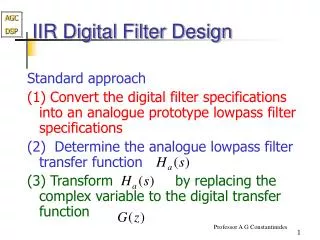
3. 10.1.1 Basic Approaches to design FIR filters • Unlike IIR digital filter design, FIR filter design does not have any connection with the design of analog filters. • The design of FIR filters is based on a direct approximation of the specified magnitude response, with often added requirement that the phase response be linear.

4. Recall a causal FIR frequency response H(e jω) of length N+1: Magnitude Response Phase Response • For a linear-phase FIR, we have: • Or, as we known:h[n] = ± h[N-n] For β= 0,π, ±π/2

5. 10.1.2 Estimation of the Filter Order • The order (length-1) of G(z) is directly estimated from the digital filter specification. Several authors have advanced formulas : • Kaiser’s Formula: • Bellanger’s Formula:

6. Estimation of the Filter Order • Hermann’s Formula: a1=0.005309, a2=0.07114, a3=-0.4761, a4=0.00266, a5=0.5941, a6=0.4278, b1=11.01217, b2=0.51244

7. A Comparison of FIR Filter Order Formulas: (1) Each of these three formulas provide only an estimate of the required filter order. (1) The estimated filter order N of the FIR filter is inversely proportionalto the transition band width (ωp-ωs ). And does not depend on the actual location of the transition band. (3) The order of Kaiser’s and Bellanger’s formulas depends on the productδpand δs. (4) Each one of three formulas can also be used to estimate the order of highpass, bandpass and bandstop FIR filter. (5) For two transition bands, we always use the smallest width to compute the order of the filter.

8. 10.2 FIR Filter Design Based on Windowed Fourier Series • Two direct approaches to design of FIR filters: (1) Truncating the Fourier series representation of the prescribed frequency response. (direct and straightforward) (2) Sampling the frequency response to get the DFT of h[n], and use IDFT to get h[n].

9. 10.2.1 Least Integral-Squared Error Design of FIR Filters • Let Hd(ejω) denotes the desired frequency response function, hd[n] denotes the impulse response samples, so : Fourier series In most application, for meeting the FR Hd(ejω) requirements, hd[n] is infinite.

10. We want to find: a Length-N, causal So: The procedure of using ht[n] to replace hd[n] is called truncating or windowing. Using what approximating criterion? Minimum Integral-Squared Error.

11. Best finite-length approximation to ideal infinite-length impulse response in the mean-square sense is obtained by truncation. • Define integral-squared error: Using Parseval’s relation, we get: When ht[n]=hd[n] for -M≤n≤M, the ΦR is minimum.

12. A causal FIR filter with an impulse response h[n] can be derived from ht[n] by delaying: The causal FIR filter h[n] has the same magnitude response as ht[n] and its phase response has a linear phase shift of ωM radians with respect to that of ht[n]. • h[n]---- linear phase • ht[n]----zero phase

13. 10.2.2 Impulse Responses of Ideal Filters • Ideal lowpass filter: • Ideal highpass filter:

14. Ideal bandpass filter: • Ideal bandstop filter:

15. Hilbert transformer (90-degree phase shifter)

16. Differentiator:

17. Truncate the h[n] of Ideal Lowpass Filter • The impulse response of ideal filter is infinite. By setting all coefficients outside the range -M≤ n ≤ M equal to zero, we arrive at a finite-length sequence. • And by shifting to the right yields the causal FIR lowpass filter which we need. • Note: In above expression, length N is 2M+1.

19. 10.2.3 Gibbs Phenomenon-- The Effect of Truncating the h[n] • Gibbs phenomenon - Oscillatory behavior in the magnitude responses of causal FIR filters obtained by truncating the impulse response coefficients of ideal filter

20. where and are the DTFTs of and , respectively. Gibbs Phenomenon Interpretation: truncating operation  windowing operation: In the frequency domain:

21. A rectangular window is used to achieve simple truncation: main lobe Width: 4π/(2M+1) side-lobes

22. Thus is obtained by a periodic continuous convolution of with

23. As can be seen, as the length of the lowpass filter is increased, the number of ripples in both passband and stopband increases, with a corresponding decrease in the ripple widths; • Height of the largest ripples remain the same independent of length; Gibbs phenomenon • Area under each lobe remains constant while width of each lobe decreases with an increase in M. • Similar oscillatory behavior observed in the magnitude responses of the truncated versions of other types of ideal filters.

24. Increasing the truncation-length of window can decrease the width of the transition band, but can’t change the relative value of the main-lobe and side-lobes. • So,we need a window: (1) It’s main lobe width is as narrow as possible to ensure a fast transition from passband to stopband. (2) Reducing the relative magnitude of the maximum sidelobe to reduce the passband and stopband ripple.

25. Rectangular window has an abrupt transition to zero outside the range • -M≤n≤M , which results in Gibbs phenomenon in • Gibbs phenomenon can be reduced either: (1) Using a window that tapers smoothly to zero at each end; (2) Providing a smooth transition from passband to stopband in the magnitude specifications.

26. Rectangular window 0 -20 -40 Gain, dB -60 -80 -100 0 0.2 0.4 0.6 0.8 1 w p / 10.2.4 Fixed Window Functions • Rectangular window

27. Hanning window 0 -20 -40 Gain, dB -60 -80 -100 0 0.2 0.4 0.6 0.8 1 w p / • Hanning window

28. Hamming window 0 -20 -40 Gain, dB -60 -80 -100 0 0.2 0.4 0.6 0.8 1 w p / • Hamming window:

29. Blackman window 0 -20 -40 Gain, dB -60 -80 -100 0 0.2 0.4 0.6 0.8 1 w p / • Blackman window:

30. Performance of a window function in LPF design • Magnitude spectrum of each window characterized by a main lobe centered at w = 0 followed by a series of sidelobes with decreasing amplitudes. • Parameters predicting the performance of a window in filter design are: • Main lobe width --- ML • Relative sidelobe level --- Asl • given by the difference in dB between amplitudes of largest sidelobe and main lobe.

31. Observe • Thus, • Passband and stopband ripples are same.

32. Distance between the locations of the maximum passband deviation and minimum stopband value  ML • Width of transition band: w = s - p < ML • To ensure a fast transition from passband to stopband, window should have a very small main lobe width. • To reduce the passband and stopband ripple d, the area under the sidelobes should be very small. • Unfortunately, these two requirements are contradictory.

33. Rectangular and Blackman windows

34. In the case of rectangular, Hann, Hamming, and Blackman windows, the value of ripple does not depend on filter length or cutoff frequency c, and is essentially constant. • In addition, w  c / M where c is a constant for most practical purposes. So, we can determine w by M.

35. Table 10.2 Properties of some fixed window functions

36. Rectangular window Hanning window 0 0 -20 -20 -40 Gain, dB Gain, dB -40 -60 -60 -80 -80 -100 -100 0 0.2 0.4 0.6 0.8 1 0 0.2 0.4 0.6 0.8 1 w p / w p / Hamming window Blackman window 0 0 -20 -20 -40 -40 Gain, dB Gain, dB -60 -60 -80 -80 -100 -100 0 0.2 0.4 0.6 0.8 1 0 0.2 0.4 0.6 0.8 1 w p w p / / • Plots of magnitudes of the DTFTs of these windows for M = 25 are shown below:

37. 10.2.5 Adjustable Window Functions • Kaiser window Where: We can adjust b to modify the window function. So, it is called as adjustable window function. Equation(10.41) and (10.42) give how to get b and N.

38. Dolph-Chebyshev window Where, g is the relative sidelobe amplitude.

39. Example of FIR Filter Design: Design a linear phase FIR LPF: • If given the passband edge frequency ωp=0.3π, the passband ripple is 1dB，the stopband edge frequency ωs=0.5π, the minimum stopband attenuation <-40dB. • Solution: αp =1dB, αs=40dB

40. The ideal LP impulse response is: If we select window Hann, calculate order N: Select a window based on table 10.2 and specifications: αs=40dB;

41. If we select window Hamming: If we select window Blackman: If we select window Kaiser:

42. FIR Filter Design Example 1 • The specifications of a low pass filter: Pass band edge 400Hz Stop band edge 1650Hz Stop band attenuation 50dB Sampling frequency 11.025kHz

43. Transition width △f = 1650-400 = 1250Hz • Another parameter fc = (400+1650)/2 = 1025 Hz, So • Choose Hamming window (-54dB),

44. ∴ N=2M+1=31 • The finite-length causal FIR LP filter:

45. The Hamming window is • So,h[n]of the filter which we need is • Then the magnitude response and the impulse response are drawn in next silde:

46. So, the original sound: the output sound after passing the LP filter:

47. FIR Filter Design Example 2 • The specifications of a high pass filter: Pass band edge 1650Hz Stop band edge 400Hz Stop band attenuation 50dB Sampling frequency 11.025kHz

48. Transition width △f = 1650-400 = 1250Hz • Another parameter fc = (400+1650)/2 = 1025 Hz, • Choose Hamming window (-54dB),

49. ∴ N=2M+1=31 • The finite-length causal FIR HP filter:

50. The Hamming window is ( no change ) • So,h[n]of the filter which we need is • Then the magnitude response and the impulse response are drawn in next silde: