Download
1 / 22
220 likes | 390 Vues
Amplification Mechanisms in Liquidity Crises. Arvind Krishnamurthy Northwestern University. Amplification. Losses on Subprime Mortgages (Fall 07 est.) At most $500 bn Decline in world stock market (Sep 08 to Oct 08) Close to $26,000 bn Expected output losses (IMF forecast) $4,700 bn.

E N D
Amplification Mechanisms in Liquidity Crises Arvind Krishnamurthy Northwestern University
Amplification • Losses on Subprime Mortgages (Fall 07 est.) • At most $500 bn • Decline in world stock market (Sep 08 to Oct 08) • Close to $26,000 bn • Expected output losses (IMF forecast) • $4,700 bn
Amplification Mechanisms • I am going to describe two financial mechanisms that have played an important role in the crisis • Balance sheet amplification • Uncertainty amplification • I omit … • Subprime was the trigger for a real estate bubble bursting • Aggregate demand effects
Liquidity model • Investors (continuum) A and B own one unit of an asset at date s • Intermediary (bank/market-maker/trading desk) provides price support at date t>s: • Promises to provide liquidity to sellers at P=1 • But, Bank has only 2 > L > 1 units of liquidity • Investors may receive shocks that require them to liquidate: • φA , φB
Fundamental equilibrium at date t • One of four states • No shocks: P = 1 • A shock: P = 1 • B shock: P = 1 • A and B shocks: P = L/2 • Date s price: • Ps = 1 – (1 – L/2) φAφB • Liquidity discount = (1 – L/2) φAφB
Balance Sheet Considerations • Define the “equity net worth” of an investor as W = Pt – Ds • Suppose date t holdings are subject to a capital/collateral constraint m Θt < W • 1 – Θt is amount liquidated if constraint binds: 1 – Θt = 1 - (Pt – Ds) /m
Consider states (A) or (B) • P = 1 is equilibrium if L is small • If Ds is large, liquidation curve shifts up and right • Or, larger fundamental liquidity shock, liquidation curve shifts up and right • Or, m increases, twists liquidation function • All cases, multiple equilibria E1 Pt = 1 E2 E3 Lt = 1 – (Pt - Ds)/2m Lt
Policy Response: Add liquidity (increase L) E1 Pt = 1 E2 Lt = 1 – (Pt - ds)/2m E3 Lt
Policy Response: Discount loans at m* < m E1 Pt = 1 E2 Lt = 1 – (Pt - ds)/2m E3 Lt
Policy Response: Buy distressed assets E1 Pt = 1 E2 Lt = 1 – (Pt - ds)/2m E3 Lt
Crisis Policy • Liquidity injection • Buying troubled assets • Discount lending • Equity injections …
Ex-ante Policy • If we push the model further (I wont here), there is another policy that pops up: • Ex-post externalities that agents don’t internalize ex-ante • Over-leveraging in the financial sector • Ex-ante leverage limitation.
Recap • So far, liquidation model • Next, Uncertainty and Crises
Uncertainty • Subprime crisis: • Complex CDO products, splitting cash flows in unfamiliar ways • Substantial uncertainty about where the losses lie • But less uncertainty about the direct aggregate loss (small) • Knightian uncertainty, ambiguity aversion, uncertainty aversion, robustness preferences
Modeling: • Standard expected utility • max{c} EP u(c) • P refers to the agent’s subjective probability distribution • Modeling ambiguity/uncertainty/robustness: • max{c}min{Q ϵQ }EQ u(c) • Q is the set of probability distributions that the agent entertains
Uncertainty in the baseline model • Recall, agents may receive liquidity shocks that makes them sell assets at date t • Shock probabilities are φA , φB • Suppose agents are uncertain about the correlation between their liquidity shocks of A and B. • ρ (A,B) ϵ [0, 1]
Worst-case decision rules • max{c}min{Q ϵQ }EQ u(c) Worst-cases for A (and B) is ρ (A,B) = 1 • Agents subjective probs only consider two states • No shocks: P = 1 • A and B shocks together: P = L/2 • Date s price: • Ps = 1 – (1 – L/2) φ • Liquidity discount = (1 – L/2) φ
Compare to baseline case • One of four states • No shocks: P = 1 • A shock: P = 1 • B shock: P = 1 • A and B shocks: P = L/2 • Date s price: • Ps = 1 – (1 – L/2) φAφB • Liquidity discount = (1 – L/2) φAφB • Uncertainty magnifies the importance of the liquidation event: order(φ) versus order(φ2)
Crisis Policy • LLR policy again • Inject liquidity into bank in the event that both shocks hit. • Liquidity discount = (1 – L/2) φ • Larger effect on agent’s uncertainty, but CB delivers only with probability φAφB
Ex-ante Policy • In liquidity externality model, it was to reduce date s leverage • More generally, this is about incentivizing better ex-ante risk management • But does the central bank really know better? • Especially when it comes to new financial products • History … everyone is blindsided in the same way
Ex-ante Policy • Policing new innovations, these are the trouble spots • Regulations slow new innovations
Summary • Two financial amplification mechanisms • Interactions • Crisis policies are similar • Ex-ante policies are different • Regulate leverage of financial sector • Regulate growth in particular of financial innovation