Download

1 / 36
360 likes | 382 Vues
Learn how normal distributions and statistical inference can be used to predict the outcomes of coin toss experiments. Explore the honest-coin and dishonest-coin principles and apply the 68-95-99.7 rule to make reasonable predictions.

E N D
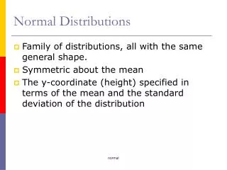
16 Mathematics of Normal Distributions 16.1 Approximately Normal Distributions of Data 16.2 Normal Curves and Normal Distributions 16.3 Standardizing Normal Data 16.4 The 68-95-99.7 Rule 16.5 Normal Curves as Models of Real-Life Data Sets 16.6 Distribution of Random Events 16.7 Statistical Inference
Statistical Inference Supposethat we have an honest coin and intend to toss it 100 times. We are going to dothis just once, and we will let X denote the resulting number of heads. Been there,done that! What’s new now is that we a have a solid understanding of the statisticalbehavior of the random variable X–it has an approximately normal distributionwith mean = 50and standard deviation = 5–and this allows us to makesome very reasonable predictions about the possible values of X.
Statistical Inference For starters, we can predict the chance that X will fall somewhere between 45and 55 (one standard deviation below and above the mean)–it is 68%. Likewise,we know that the chance that X will fall somewhere between 40 and 60 is 95%,and between 35 and 65 is a whopping 99.7%. What if, instead of tossing the coin 100 times, we were to toss it n times?
Statistical Inference Not surprisingly, bell-shaped distribution would still be there–only thevalues of and would change. Specifically, for n sufficiently large (typicallyn ≥ 30), the number of heads in n tosses would be a random variable with an approximately normal distribution with mean = n/2 heads and standard deviation heads. This is an important fact for which we have coined thename the honest-coin principle.
THE HONEST-COIN PRINCIPLE Let X denote the number of heads in n tosses of an honest coin (assumen ≥ 30). Then, X has an approximately normaldistribution with mean = n/2 and standard deviation
Example 16.9 Coin-Tossing Experiments: Part 2 An honest coin is going to be tossed 256 times. Before this is done, we have theopportunity to make some bets. Let’s say that we can make a bet (with evenodds) that if the number of heads tossed falls somewhere between 120 and 136,we will win; otherwise, we will lose. Should we make such a bet? Let X denote the number of heads in 256 tosses of an honest coin.
Example 16.9 Coin-Tossing Experiments: Part 2 By thehonest-coin principle, X is a random variable having a distribution that is approxi-mately normal with mean = 256/2 = 128 heads and standard deviationheads. The values 120 to 136 are exactly one standard deviation below and above the mean of 128, which means that there is a 68% chancethat the number of heads will fall somewhere between 120 and 136.
Example 16.9 Coin-Tossing Experiments: Part 2 We should indeed make this bet! A similar calculation tells us that there is a 95% chance thatthe number of heads will fall somewhere between 112 and 144, and the chance thatthe number of heads will fall somewhere between 104 and 152 is 99.7%.
Dishonest Coin What happens when the coin being tossed is not an honest coin? Surprisingly,the distribution of the number of heads X in n tosses of such a coin is still approximately normal, as long as the number n is not too small (a good rule of thumb isn ≥ 30). All we need now is a dishonest-coin principle to tell us how to find themean and the standard deviation.
THE DISHONEST-COIN PRINCIPLE Let X denote the number of heads in n tosses of a coin (assume n ≥ 30). Letp denote the probability of heads on each toss of the coin. Then,X has anapproximately normal distribution with mean = n • P and standard deviation
Example 16.10 Coin-Tossing Experiments: Part 3 A coin is rigged so that it comes up heads only 20% of the time (i.e., p = 0.20).The coin is tossed 100 times (n = 100) and X is the number of heads in the 100tosses. What can we say about X?
Example 16.10 Coin-Tossing Experiments: Part 3 According to the dishonest-coin principle, the distribution of the randomvariable X is approximately normal with meanm = 100 0.20 = 20 and standard deviation Applying the 68-95-99.7 rule with = 20and = 4 gives the following facts:
Example 16.10 Coin-Tossing Experiments: Part 3 ■There is about a 68% chance that X will be somewhere between 16 and 24( – ≤ X ≤ + ). ■There is about a 95% chance that X will be somewhere between 12 and 28( – 2 ≤ X ≤ + 2 ). ■The number of heads is almost guaranteed (about 99.7%) to fall somewhere between 8 and 32 ( – 3 ≤ X ≤ + 3 ).
Example 16.10 Coin-Tossing Experiments: Part 3 In this example, heads and tails are no longer interchangeableconcepts–heads is an outcome with probability p = 0.20 while tails is an outcome with much higher probability (0.8). We can, however, apply the principleequally well to describe the distribution of the number of tails in 100 coin tosses of the same dishonest coin: The distribution for the number of tails isapproximately normal with mean = 100 0.80 = 80 and standard deviation
Central Limit Theorem The dishonest-coin principle is a special version of one of the most importantlaws in statistics, a law generally known as the central limit theorem. We will nowbriefly illustrate why the importance of the dishonest-coin principle goes beyondthe tossing of coins.
Example 16.11 Sampling for Defective Light Bulbs An assembly line produces 100,000 light bulbs a day, 20% of which generallyturn out to be defective. Suppose that we draw a random sample of n = 100 light bulbs. Let X represent the number of defective light bulbs in the sample.What can we say about X? A moment’s reflection will show that, in a sense, this example is completelyparallel to Example 16.10–think of selecting defective light bulbs as analogousto tossing heads with a dishonest coin.
Example 16.11 Sampling for Defective Light Bulbs We can use the dishonest-coin principle toinfer that the number of defective light bulbs in the sample is a randomvariable having an approximately normal distribution with a meanof 20 light bulbs and standard deviation of 4 light bulbs. Usingthese facts, we can draw the following conclusions:
Example 16.11 Sampling for Defective Light Bulbs ■ There is a 68% chance that the number of defective lightbulbs in the sample will fall somewhere between 16 and 24. ■ There is a 95% chance that the number of defective lightbulbs in the sample will fall somewhere between 12 and 28. ■ The number of defective light bulbs in the sample is practicallyguaranteed (a 99.7% chance) to fall somewhere between 8 and 32.
Example 16.11 Sampling for Defective Light Bulbs Probably the most important point here is that each of the preceding facts can be rephrased in terms of sampling errors (Chapter 13). For example, say we had 24 defective light bulbs in the sample; in other words, 24% of the sample (24 out of 100)are defective light bulbs. If we use this statistic to estimate the percentage of defective light bulbs overall, then the sampling error would be 4% (because theestimate is 24% and the value of the parameter is 20%).
Example 16.11 Sampling for Defective Light Bulbs By the same token, if wehad 16 defective light bulbs in the sample, the sampling error would be –4%. Coincidentally, the standard deviation is = 4 light bulbs, or 4% of the sample. (Wecomputed it in Example 16.10.) Thus, we can rephrase our previous assertionsabout sampling errors as follows:
Example 16.11 Sampling for Defective Light Bulbs ■When estimating the proportion of defective light bulbs coming out of the assembly line by using a sample of 100 light bulbs, there is a 68% chance thatthe sampling error will fall somewhere between –4% and 4%.
Example 16.11 Sampling for Defective Light Bulbs ■When estimating the proportion of defective light bulbs coming out of the assembly line by using a sample of 100 light bulbs, there is a 95% chance thatthe sampling error will fall somewhere between –8% and 8%.
Example 16.11 Sampling for Defective Light Bulbs ■When estimating the proportion of defective light bulbs coming out of the assembly line by using a sample of 100 light bulbs, there is a 99.7% chance thatthe sampling error will fall somewhere between –12% and 12%.
Example 16.12 Sampling with Larger Samples Suppose that we have the same assembly line as in Example 16.11, but this time weare going to take a really big sample of n = 1600light bulbs. Before we even countthe number of defective light bulbs in the sample, let’s see how much mileage wecan get out of the dishonest-coin principle. The standard deviation for the distribution of defective light bulbs in the sample is
Example 16.12 Sampling with Larger Samples which justhappens to be exactly 1% of the sample (16/1600 = 1%). This means that whenwe estimate the proportion of defective light bulbs coming out of the assembly lineusing this sample, we can have some sort of a handle on the sampling error.
Example 16.12 Sampling with Larger Samples ■We can say with some confidence (68%) that the sampling error will fallsomewhere between –1% and 1%. ■We can say with a lot of confidence (95%) that the sampling error will fallsomewhere between –2% and 2%. ■We can say with tremendous confidence (99.7%) that the sampling error willfall somewhere between –3% and 3%.
Example 16.13 Measuring the Margin of Error of a Poll In California, school bond measures require a 66.67% vote for approval. Supposethat an important school bond measure is on the ballot in the upcoming election.In the most recent poll of 1200 randomly chosen voters, 744 of the 1200 voterssampled, or 62%, indicated that they would vote for the school bond measure.Let’s assume that the poll was properly conducted and that the 1200 voters sampled represent an unbiased sample of the entire population.
Example 16.13 Measuring the Margin of Error of a Poll What are the chancesthat the 62% statistic is the result of sampling variability and that the actual votefor the bond measure will be 66.67% or more? Here, we will use a variation of the dishonest-coin principle, with eachvote being likened to a coin toss: A vote for the bond measure is equivalent toflipping heads, a vote against the bond measure is equivalent to flipping tails.
Example 16.13 Measuring the Margin of Error of a Poll In this analogy, the probability (p) of “heads” represents the proportion of voters in the population that support the bond measure: If p turns out to be 0.6667 ormore, the bond measure will pass. Our problem is that we don’t know p, so howcan we use the dishonest-coin principle to estimate the mean and standard deviation of the sampling distribution?
Example 16.13 Measuring the Margin of Error of a Poll We start by letting the 62% (0.62) statistic from the sample serve as an estimate for the actual value of p in the formula for the standard deviation given bythe dishonest-coin principle. (Even though we know that this is only a rough estimate for p, it turns out to give us a good estimate for the standard deviation .)
Example 16.13 Measuring the Margin of Error of a Poll Using p = 0.62 and the dishonest-coin principle, we get votes. This number represents the approximate standard deviation for the number of“heads”(i.e., voters who will vote for the school bond measure) in the sample.
Example 16.13 Measuring the Margin of Error of a Poll If weexpress this number as a percentage of the sample size, we can say that the standarddeviation represents approximately 1.4% of the sample (16.8/1200 = 0.014). The standard deviation for the sampling distribution of the proportion ofvoters in favor of the measure expressed as a percentage of the entire sample iscalled the standard error. (For our example, we have found above that the standarderror is approximately 1.4%.)
Example 16.13 Measuring the Margin of Error of a Poll In sampling and public opinion polls, it is customaryto express the information about the population in terms of confidence intervals,which are themselves based on standard errors: A 95% confidence interval isgiven by two standard errors below and above the statistic obtained from thesample, and a 99.7% confidence interval is given by going three standard errorsbelow and above the sample statistic.
Example 16.13 Measuring the Margin of Error of a Poll For the school bond measure, a 95% confidence interval is 62% plus orminus2 (1.4%)= 2.8%. This means that we can say with 95% confidence (wewould be right approximately 95 out of 100 times) that the actual vote for thebond measure will fall somewhere between 59.2% (62 – 2.8) and 64.8% (62 + 2.8) and thus that the bond measure will lose.
Example 16.13 Measuring the Margin of Error of a Poll Take a 99.7% confidence interval of 62% plus or minus 3 (1.4%)=4.2%–itis almost certain that the actual vote will turn out somewhere in that range. Evenin the most optimistic scenario, the vote will not reach the 66.67% needed to passthe bond measure.