Hidden Markov Models Outline
Hidden Markov Models Outline. Markov models Hidden Markov models Forward/Backward algorithm Viterbi algorithm Baum-Welch estimation algorithm. Markov Models. Observable states: 1,2, … ,N Observable sequence: q 1 ,q 2 , … ,q t , … ,q T

Hidden Markov Models Outline
E N D
Presentation Transcript
Hidden Markov ModelsOutline • Markov models • Hidden Markov models • Forward/Backward algorithm • Viterbi algorithm • Baum-Welch estimation algorithm 236607 Visual Recognition Tutorial
Markov Models • Observable states: 1,2,…,N • Observable sequence: q1 ,q2 ,…,qt ,…,qT • First order Markov assumption: • Stationarity: 236607 Visual Recognition Tutorial
Markov Models • State transition matrix A: where • Constraints on : 236607 Visual Recognition Tutorial
Markov Models: Example • States: • Rainy (R) • Cloudy (C) • Sunny (S) • State transition probability matrix: • Compute the probability of observing SSRRSCS given that today is S. 236607 Visual Recognition Tutorial
Markov Models: Example • Basic conditional probability rule: • The Markov chain rule: 236607 Visual Recognition Tutorial
Markov Models: Example • Observation sequence O: • Using the chain rule we get: 236607 Visual Recognition Tutorial
Markov Models: Example • What is the probability that the sequence remains in state i for exactly d time units? • Exponential Markov chain duration density. • What is the expected value of the duration d in state i? 236607 Visual Recognition Tutorial
Markov Models: Example 236607 Visual Recognition Tutorial
Markov Models: Example • Avg. number of consecutive sunny days = • Avg. number of consecutive cloudy days = 2.5 • Avg. number of consecutive rainy days = 1.67 236607 Visual Recognition Tutorial
Hidden Markov Models • States are not observable • Observations are probabilistic functions of state • State transitions are still probabilistic 236607 Visual Recognition Tutorial
Urn and Ball Model • N urns containing colored balls • M distinct colors of balls • Each urn has a (possibly) different distribution of colors • Sequence generation algorithm: • Pick initial urn according to some random process. • Randomly pick a ball from the urn and then replace it • Select another urn according a random selection process asociated with the urn • Repeat steps 2 and 3 236607 Visual Recognition Tutorial
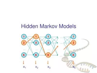
The Trellis N 4 3 2 1 STATES 1 2 t-1 t t+1 t+2 T-1 T TIME o1 o2 ot-1 ot ot+1 ot+2 oT-1 oT OBSERVATION 236607 Visual Recognition Tutorial
Elements of Hidden Markov Models • N– the number of hidden states • Q– set of states Q={1,2,…,N} • M– the number of symbols • V– set of symbols V ={1,2,…,M} • A– the state-transition probability matrix • B – Observation probability distribution: • p - the initial state distribution: • l – the entire model 236607 Visual Recognition Tutorial
Three Basic Problems • EVALUATION– given observation O=(o1 , o2 ,…,oT ) and model , efficiently compute • Hidden states complicate the evaluation • Given two models l1 and l1, this can be used to choose the better one. • DECODING - given observation O=(o1 , o2 ,…,oT ) and model l find the optimal state sequence q=(q1 , q2 ,…,qT ) . • Optimality criterion has to be decided (e.g. maximum likelihood) • “Explanation” of the data. • LEARNING– given O=(o1 , o2 ,…,oT ), estimate model parameters that maximize 236607 Visual Recognition Tutorial
Solution to Problem 1 • Problem: Compute P(o1 , o2 ,…,oT |l). • Algorithm: • Let q=(q1 , q2 ,…,qT ) be a state sequence. • Assume the observations are independent: • Probability of a particular state sequence is: • Also, 236607 Visual Recognition Tutorial
Solution to Problem 1 • Enumerate paths and sum probabilities: • N T state sequences and O(T) calculations. Complexity: O(T N T) calculations. 236607 Visual Recognition Tutorial
Forward Procedure: Intuition N 3 2 1 aNk STATES a3k k v a1k t t+1 TIME 236607 Visual Recognition Tutorial
Forward Algorithm • Define forward variable as: • is the probability of observing the partial sequence such that the state qtis i. • Induction: • Initialization: • Induction: • Termination: • Complexity: 236607 Visual Recognition Tutorial
Example • Consider the following coin-tossing experiment: • state-transition probabilities equal to 1/3 • initial state probabilities equal to 1/3 • You observe O=(H,H,H,H,T,H,T,T,T,T). What state 236607 Visual Recognition Tutorial
Example • You observe O=(H,H,H,H,T,H,T,T,T,T). What state sequence q, is most likely? What is the joint probability, , of the observation sequence and the state sequence? • What is the probability that the observation sequence came entirely of state 1? • Consider the observation sequence • How would your answers to parts 1 and 2 change? 236607 Visual Recognition Tutorial
Example • If the state transition probabilities were: How would the new model l’ change your answers to parts 1-3? 236607 Visual Recognition Tutorial
Backward Algorithm N 4 3 2 1 STATES 1 2 t-1 t t+1 t+2 T-1 T TIME o1 o2 ot-1 ot ot+1 ot+2 oT-1 oT OBSERVATION 236607 Visual Recognition Tutorial
Backward Algorithm • Define backward variable as: • is the probability of observing the partial sequence such that the state qtis i. • Induction: 1. Initialization: 2. Induction: 236607 Visual Recognition Tutorial
Solution to Problem 2 • Choose the most likely path • Find the path (q1 , q2 ,…,qT ) that maximizes the likelihood: • Solution by Dynamic Programming • Define • is the highest prob. Path ending in state I • By induction we have: 236607 Visual Recognition Tutorial
Viterbi Algorithm N 4 3 2 1 aNk k STATES a1k 1 2 t-1 t t+1 t+2 T-1 T TIME o1 o2 ot-1 ot ot+1 ot+2 oT-1 oT OBSERVATION 236607 Visual Recognition Tutorial
Viterbi Algorithm • Initialization: • Recursion: • Termination: • Path (state sequence) backtracking: 236607 Visual Recognition Tutorial
Solution to Problem 3 • Estimate to maximize • No analytic method because of complexity – iterative solution. • Baum-Welch Algorithm (actually EM algorithm) : • Let initial model be l0 • Compute new l based on l0 and observation O. • If • Else set l0 l and go to step 2 236607 Visual Recognition Tutorial
Baum-Welch: Preliminaries • Define as the probability of being in state i at time t, and in state j at time t+1. • Define as the probability of being in state i at time t, given the observation sequence 236607 Visual Recognition Tutorial
Baum-Welch: Preliminaries • is the expected number of times state i is visited. • is the expected number of transitions from state i to state j. 236607 Visual Recognition Tutorial
Baum-Welch: Update Rules • expected frequency in state i at time (t=1) • (expected number of transitions from state i to state j) / expected number of transitions from state i): • (expected number of times in state j and observing symbol k) / (expected number of times in state j ): 236607 Visual Recognition Tutorial
Properties • Covariance of the estimated parameters • Convergence rates 236607 Visual Recognition Tutorial
Types of HMM • Continuous density • Ergodic • State duration 236607 Visual Recognition Tutorial
Implementation Issues • Scaling • Initial parameters • Multiple observation 236607 Visual Recognition Tutorial
Comparison of HMMs • What is natural distance function? • If is large, does it mean that the models are really different? 236607 Visual Recognition Tutorial
References • L. Rabiner and B. Juang. An introduction to hidden Markov models. IEEE ASSP Magazine, p. 4--16, Jan. 1986. • Thad Starner, Joshua Weaver, and Alex Pentland Machine Vision Recognition of American Sign Language Using Hidden Markov Model • Thad Starner, Alex PentlandVisual Recognition of American Sign Language Using Hidden Markov Models. In International Workshop on Automatic Face and Gesture Recognition, pages 189--194, 1995. http://citeseer.nj.nec.com/starner95visual.html 236607 Visual Recognition Tutorial


