Discrete Transform
Discrete Transform. Introduction. A transform maps image data into a different mathematical space via a transformation equation. One example of transform that we had encountered before is the transform from one color space to another color space. RGB to SCT (spherical coordinate transform).


Discrete Transform
E N D
Presentation Transcript
Introduction • A transform maps image data into a different mathematical space via a transformation equation. • One example of transform that we had encountered before is the transform from one color space to another color space. • RGB to SCT (spherical coordinate transform). • RGB to HSL (hue/saturation/lightness).
Introduction • However, the transform from one color space to another color space has a one-to-one correspondence between a pixel in the input and the output. • Here, we are mapping the image data from the spatial domain to the frequency domain (spectral domain).
Introduction • All the pixels in the input (spatial domain) contribute to each value in the output (frequency domain). (see fig. 5.1.1). • Discrete transforms are performed based on specific functions, which are called the basis functions. • These functions are typically sinusoidal or rectangular. • The discrete version of 1-D basis function are called basis vectors. (see fig. 5.1.2). • The discrete version of 2-D basis function are called basis images (or basis matrices). (see fig. 5.1.1(c)).
Introduction • The process of transforming the image data into another domain involves projecting the image onto the basis images • The mathematical term for this projection process is called an inner product. • This is identical to what we have done with Frei-Chen masks. • Assuming an NxN image, the general form of the transformation equation is as follows: See fig: 5.1.5
Introduction • u and v are the frequency domain coordinates. • T(u,v) are the transform coefficients. • B(r,c;u,v) are the basis images, corresponding to each different value for u and v, and the size of each is r x c.
Introduction • The transform coefficients T(u,v) are the projection of I(r,c) onto each B(u,v). • These coefficients tell us how similar the image is to the basis image. • The more alike they are, the bigger the coefficients. • The transformation process composed the image into a weighted sum of basis images where T(u,v) are the weights. See eg: 5.1.1
Introduction • To obtain the image from the transform coefficients, we apply the inverse transform equation: See eg: 5.1.2
Introduction • Here, the B-1(r,c;u,v) represents the inverse basis images. • In many cases, the inverse basis images are the same as the forward ones, but possibly weighted by a constant. • Here, we will learn 3 types of transforms: • Walsh-Hadamard Transform, Fourier Transform and Cosine Transform.
Walsh-Hadamard Transform • For Walsh-Hadamard, the basis functions are based on square or rectangular waves with peaks of +1 and -1. • One main advantage of rectangular basis functions is that the computations are very simple. • When we project the image onto the basis functions, all we need to do is to multiply each pixel with +1 or -1.
Walsh-Hadamard Transform • Depending on the size of the image to be transformed, we must use basis images with the right size. • To convert an NxN image, we need to use a set of NxN basis images. • For example, to transform a 2x2 image, then we need to use the set of 2x2 basis images as shown in the next slide.
Walsh-Hadamard Transform The set of 2x2 Walsh-Hadamard basis images
Walsh-Hadamard Transform • Once we have the basis images, we can perform the transform operation to convert an image from the spatial domain to the frequency domain. • Project the image onto each of the basis images. • The result should be a matrix that has the same size as the image. • This is the frequency domain of that image.
Walsh-Hadamard Transform • The equation for the whole transform operation is given below: • In this case, N refers to the dimension of the image.
Walsh-Hadamard Transform • To reconstruct the original image from the transform coefficients, we need to perform an inverse transform operation. • The equation is as follows:
Walsh-Hadamard Transform • From the equation, it can be seen that the inverse basis images is just the same as the forward basis images. • It means that the original image can be obtained by taking the transform coefficients and run it through the same operation as the one for forward transform.
Walsh-Hadamard Transform • The difference between the different types of transform is the basis images used. • Each type of transform has its own equation to be used to generate the basis images. • To make things easier, we will learn how to generate the basis vectors first, and using the basis vectors, we will generate the basis images.
Walsh-Hadamard Transform • Assuming an N-points basis vector, the equation to generate a 1-D Walsh-Hadamard basis vector is as follows:
Walsh-Hadamard Transform • v is the index in the frequency domain. • c is the index in the spatial domain. • N is the number of points in the basis vector. • n = log2N, which is the number of bits in the number N. • bi(c) is found by considering c as a binary number and finding the ith bit. It means the ith bit in c.
Walsh-Hadamard Transform • pi(v) is found as follows:
Walsh-Hadamard Transform • Some examples on finding the variables: • If N = 8, then n = 3, because log28 = 3. If c = 410 = 1002, then b2(c) = 1, b1(c) = 0 and b0(c) = 0. • If N = 16, then n = 4, because log216 = 4. If c = 210 = 00102, then b3(c) = 0, b2(c) = 0, b1(c) = 1 and b0(c) = 0.
v=0(002) i 0 1 c bi(c) pi(v) bi(c) pi(v) WHv(c) - n 1 å b ( c ) p ( v ) i i = i 0 0(00) 0 0 0 0 0 1 1(01) 1 0 0 0 0 1 2(10) 0 0 1 0 0 1 3(11) 1 0 1 0 0 1 Walsh-Hadamard Transform • Example: Building the 4-points Walsh-Hadamard basis vector set. • Start by finding the basis vector for v = 0. • The result is [1 1 1 1].
v=1(012) i 0 1 c bi(c) pi(v) bi(c) pi(v) WHv(c) - n 1 å b ( c ) p ( v ) i i = i 0 0(00) 0 0 0 1 0 1 1(01) 1 0 0 1 0 1 2(10) 0 0 1 1 1 -1 3(11) 1 0 1 1 1 -1 Walsh-Hadamard Transform • Next, find the basis vector for v = 1. • The result is [1 1 -1 -1].
v=2(102) i 0 1 c bi(c) pi(v) bi(c) pi(v) WHv(c) - n 1 å ( ) ( ) b c p v i i = i 0 0(00) 0 1 0 1 0 1 1(01) 1 1 0 1 1 -1 2(10) 0 1 1 1 1 -1 3(11) 1 1 1 1 2 1 Walsh-Hadamard Transform • Then, find the basis vector for v = 2. • The result should be [1 -1 -1 1].
v=3(112) i 0 1 c bi(c) pi(v) bi(c) pi(v) WHv(c) - n 1 å b ( c ) p ( v ) i i = i 0 0(00) 0 1 0 2 0 1 1(01) 1 1 0 2 1 -1 2(10) 0 1 1 2 2 1 3(11) 1 1 1 2 3 -1 Walsh-Hadamard Transform • Finally, find the basis vector for v = 3. • The result it [1 -1 1 -1].
Walsh-Hadamard Transform • Using the the 1-D basis vectors, we can generate the 2-D Walsh-Hadamard basis images. • Example: Generating the 4x4 basis image for u = 3 and v = 2. • Look at the basis vector for index 3 and 2. • For index 3: [1 -1 1 -1] • For index 2: [1 -1 -1 1]
1-D basis vector for v = 2 +1 -1 -1 +1 +1 -1 -1 +1 +1 -1 +1 +1 -1 1-D basis vector for u = 3 -1 +1 -1 -1 +1 +1 -1 +1 +1 -1 -1 Walsh-Hadamard Transform Fill in the matrix by multiplying the corresponding row and columns.
Walsh-Hadamard Transform • Remember that we need to scale the resulting matrix by 1 / √N. • In this case, N = 16, and therefore √N = 4.
Walsh-Hadamard Transform • By finding the basis images for every combination of u and v, we can get a set of Walsh-Hadamard basis images. • The set of 4x4 Walsh-Hadamard basis images are shown in the next slide. • White color corresponds to +1. • Black color corresponds to -1.
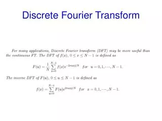
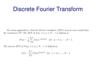
Fourier Transform • The Fourier transform is the most well known, and the most widely used, transform. • Fourier transform is used in many applications: • Vibration analysis in mechanical engineering. • Circuit analysis in electrical engineering. • Computer imaging.
Fourier Transform • Fourier transform decomposes an image into a weighted sum of 2-D sinusoidal term. • The general formula to generate the N-points 1-D Fourier basis vector set is as follows:
Fourier Transform • The equation for the Fourier basis vector can be written in two different formats because of Euler’s identity: • ejx = cos x + j sin x • Notice that the basis vector consists of complex numbers.
c 0 0 1 -j0 1 1 0 1 -j0 1 2 0 1 -j0 1 3 0 1 -j0 1 Fourier Transform • Example: Building the 4-points Fourier basis vector set. • Start by finding the basis vector for v = 0. • The result is [1 1 1 1].
c 0 0 1 -j0 1 1 0 -j -j 2 -1 -j0 -1 3 0 -(-j) j Fourier Transform • Next, find the basis vector for v = 1. • The result is [1 –j -1 j]
c 0 0 1 -j0 1 1 -1 -j0 -1 2 1 -j0 1 3 -1 -j0 -1 Fourier Transform • Then, find the basis vector for v = 2. • The result is [1 -1 1 -1]
c 0 0 1 -j0 1 1 0 -(-j) j 2 -1 -j0 -1 3 0 -j -j Fourier Transform • Finally, find the basis vector for v = 3. • The result is [1 j -1 –j].
Fourier Transform • As in Walsh-Hadamard, the 2-D Fourier basis images can be generated from the 1-D Fourier basis vector. • Example: Generating the 4x4 basis image for u = 3 and v = 2. • Look at the basis vector for index 3 and 2. • For index 3: [1 j -1 -j] • For index 2: [1 -1 1 -1]
1-D basis vector for v = 2 +1 -1 +1 -1 +1 +1 -1 +1 -1 1-D basis vector for u = 3 +j +j -j +j -j -1 -1 +1 -1 +1 -j -j +j -j +j Fourier Transform Fill in the matrix by multiplying the corresponding row and columns.
Fourier Transform • Remember that we need to scale the resulting matrix by 1 / √N. • In this case, N = 16, and therefore √N = 4.
Fourier Transform • Once all the required basis images have been obtained, then we can perform the transform operation. • The equation for Fourier transform operation is as follows:
Fourier Transform • Due to Euler’s identity, the previous equation can also be written as follows: • Since the Fourier basis images are complex, the Fourier transform coefficients F(u,v) are also complex. • Real part: cosine terms. • Imaginary part: sine terms
Fourier Transform • After we perform the transform, we can get back the original image by applying the inverse Fourier transform. • The equation for inverse Fourier transform is as follows:
Fourier Transform • Notice that in the inverse Fourier transform, the basis function used is the complex conjugate of the one used in forward transform. • The exponent sign is changed from -1 to +1. • In the sine-cosine format, this will change the sign of the imaginary component. • Therefore, it changes the phase of the basis functions
Cosine Transform • Similar to Fourier transform, cosine transform also uses sinusoidal basis functions. • The difference is that the cosine transform basis functions are not complex. • They use only cosine functions and not sine functions. • The general formula to generate the N-points 1-D cosine basis vector set is as follows:
Cosine Transform • The equation is almost the same as the previous two transforms except that the scaling factor is not the same for all the basis vectors. • Once the 1-D basis vectors have been obtained, the 2-D basis images can be generated in the same manner as in the previous transforms.