9. Regulator design with state variable feedback and observer
870 likes | 1.51k Vues
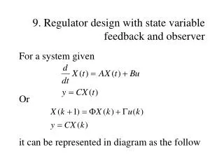
9. Regulator design with state variable feedback and observer. For a system given Or it can be represented in diagram as the follow. u(k). u(t). y(k). y(t). X (k). X (t). . B. +. C. C. +. +. +. . A. 9. Regulator design with state variable feedback and observer (cont’).

9. Regulator design with state variable feedback and observer
E N D
Presentation Transcript
9. Regulator design with state variable feedback and observer For a system given Or it can be represented in diagram as the follow
u(k) u(t) y(k) y(t) X(k) X(t) B + C C + + + A 9. Regulator design with state variable feedback and observer (cont’)
9.1 Regulator design via state variable feedback For a continuous-time system given by, suppose that all the state variables are accessible, a state variable feedback can be implemented.
9.1 Regulator design via state variable feedback (cont’) u(t) y(t) r(t) X(t) C + - KT
9.1 Regulator design via state variable feedback (cont’) This new system can be described as where KT=[k1 k2…kn] is the feedback matrix
9.1 Regulator design via state variable feedback (cont’) The transfer function for the original system is: The transfer function for the new system with state variable feedback is: That means the system performance can be improved by selecting a proper feedback matrix K.
u(k) u(k) r(k) y(k) y(k) X(k) X(k) C C + + + - KT
9.1 Regulator design via state variable feedback (cont’) The transfer function for the original system is: The transfer function for the new system with state variable feedback is: That means the system performance can be improved by selecting a proper feedback matrix K.
9.1 Regulator design via state variable feedback (cont’) For a discrete system, we have the similar conclusion. Firstly, the transfer function for the original system is: Then, the transfer function for the new system with state variable feedback is: That means the performance of the discrete system can also be improved by selecting a proper feedback matrix K.
9.1 Regulator design via state variable feedback (cont’) Example 1: Given the system transfer function as suppose 1) a state variable feedback scheme, 2) a output feedback is implemented for this system, find the closed loop transfer function and draw a diagram to show the implementation respectively. Comment on the difference of the two closed loop transfer function.
9.1 Regulator design via state variable feedback (cont’) First, find its state equations A, B and C.
9.1 Regulator design via state variable feedback (cont’) According to the controllable canonical form, we obtain: where
9.1 Regulator design via state variable feedback (cont’) Then the closed loop transfer function is:
9.1 Regulator design via state variable feedback (cont’) Finally we have: This means that the characteristic equation roots may be placed anywhere in the s-plane by choice of state variable feedback coefficients k1, k2, and k3.
9.1 Regulator design via state variable feedback (cont’) The implementation is shown as the follow: r(t) y(t) X(t) C + - KT
9.1 Regulator design via state variable feedback (cont’) First, the original system can be implemented as the follow: x3 e(t) x2 x1 y(t) + u(t) a -5 -4
9.1 Regulator design via state variable feedback (cont’) First, the original system can be implemented as the follow:
9.1 Regulator design via state variable feedback (cont’) Then, the system with state variable feedback can be implemented as the follow: -k3 x2 x3 x1 y(t) + r(t) u(t) a -5 -4 -k2 -k1
9.1 Regulator design via state variable feedback (cont’) For the system with output feedback can be implemented like this x2 x3 x1 y(t) + r(t) u(t) a -5 -4 -k1
9.1 Regulator design via state variable feedback (cont’) For the system with output feedback can be implemented like this
9.1 Regulator design via state variable feedback (cont’) For the system with output feedback can be implemented like this Tv can place its poles anywhere. However, To can’t.
9.1 Regulator design via state variable feedback (cont’) For a given continuous system, the transfer function with state variable feedback is: If the system is given as a controllable canonical for, how can we find the feedback matrix KT? First, the new system will be described as
9.1 Regulator design via state variable feedback (cont’) As the system is given as a controllable canonical form, we will have A, B and C look like
9.1 Regulator design via state variable feedback (cont’) Therefore, the new plant matrix A-BKT would be
9.1 Regulator design via state variable feedback (cont’) It still is a controllable canonical form. For this system, we can write its transfer function straight away. That is
9.1 Regulator design via state variable feedback (cont’) As for the original system, we have a transfer function as for the new (desired) system, we have the transfer function as Comparing their coefficients, we can work out the feedback matrix KT=[k1 k2… kn] straightaway.
9.1 Regulator design via state variable feedback (cont’) If the system is not given as a controllable canonical forms, we can find out the feedback matrix KT as: where P(A) is obtained by replacing the s by A in P(s). P(s) is the desired characteristic polynomial.
9.1 Regulator design via state variable feedback (cont’) For discrete system, we can have a similar conclusion. That is For this system, we can write its transfer function straight away. That is
9.1 Regulator design via state variable feedback (cont’) As for the original system, we have a transfer function as for the new (desired) system, we have the transfer function as Comparing their coefficients, we can work out the feedback matrix KT=[k1 k2… kn] straightaway.
9.1 Regulator design via state variable feedback (cont’) If the system is not given as a controllable canonical forms, we can find out the feedback matrix KT as where P() is obtained by replacing the z by in P(z). P(z) is the desired characteristic polynomial.
9.1 Regulator design via state variable feedback (cont’) Example 2: Consider the system given by Determine the state feedback gain matrix K such that the closed-loop system (regulator system) exhibits the deadbeat response to an initial state X(0).
9.1 Regulator design via state variable feedback (cont’) Obviously, this is a controllable canonical form, its transfer function is For a deadbeat system, all its poles are at ? That is
9.1 Regulator design via state variable feedback (cont’) That is, the transfer function for a system with state variable feedback is and the transfer function of the original system is
9.1 Regulator design via state variable feedback (cont’) Comparing the coefficients of the two transfer functions, we obtain
9.1 Regulator design via state variable feedback (cont’) Verification: Suppose that the initial state is given by As the new system is
9.1 Regulator design via state variable feedback (cont’) Then we have
9.1 Regulator design via state variable feedback (cont’) Exercise 1: Consider the system given by Determine the state feedback gain matrix Ksuch that the desired closed-loop poles are at , and draw a diagram to show the new system.
9.1 Regulator design via state variable feedback (cont’) Exercise 2: Consider the system given by Determine the state feedback gain matrix Ksuch that the closed-loop is a deadbeat system (Hint: using the formula for the non-controllable canonical form systems).
9.2 State observers State variable feedback system y(k) r(k) X(k) + C - KT
9.2 State observers • State observer/estimator: a subsystem in the control system that performs an estimation of the state variables based on the measurements of the output and control/input signal. • Full-order observer: an observer which estimates all n state variables regardless of whether some state variables are available from direct measurement.
9.2 State observers (cont’) • Minimum-order observer: an observer which only estimates the state variables that are not available from direct measurement. • Reduced-order observer: an observer which estimates the unmeasurable state variables and some measurable state variables.
9.2 State observers (cont’) u(k) y(k) r(k) X(k) + C + - + (State) Observer KT
9.2 State observers (cont’) Structure of an observer y(k) Ke u(k) C + +
9.2 State observers (cont’) For this observer, its inputs are the system input and output, and we need to find out the state variables. How can we design an observer?
9.2 State observers (cont’) The state equations for this observer is This observer is called a prediction observer, since the estimation is one sampling period ahead of the measurement.
9.2 State observers (cont’) The state equation for the actual system is The state equations for this observer is
9.2 State observers (cont’) We would like an observer to provide the state variable that are identical to the actual system. That is . If , then we have That is the response of the state observer system is identical to the response of the original system. How can we manage that?
9.2 State observers (cont’) For the actual system, we have For the observer system, we have If we subtract the observer from the actual system, that is
9.2 State observers (cont’) We obtain Let , then we have
9.2 State observers (cont’) For this state equation , we can draw a diagram as the follow E(k) - + C Ke