Lecture 08 State Feedback Controller Design
Lecture 08 State Feedback Controller Design. 8.1 State Feedback and Stabilization 8.2 Full-Order Observer Design 8.3 Separation Principle 8.4 Reduced-Order Observer 8.5 State Feedback Control Design with Integrator. State Feedback and Stabilization.

Lecture 08 State Feedback Controller Design
E N D
Presentation Transcript
Lecture 08 State Feedback Controller Design 8.1 State Feedback and Stabilization 8.2 Full-Order Observer Design 8.3 Separation Principle 8.4 Reduced-Order Observer 8.5 State Feedback Control Design with Integrator Modern Control Systems
State Feedback and Stabilization Stabilization by State Feedback: Regulator Case Plant: State Feedback Law: Closed-Loop System: Theorem Given Controllable There exists a state feedback matrix, F, such that Modern Control Systems
D B C A F State Feedback System (Regulator Case) Modern Control Systems
State Feedback Design in Controllable Form (8.1) Modern Control Systems
Suppose the desired characteristic polynomial (8.2) Comparing (8.1) and (8.2), we have (8.3) Modern Control Systems
State Feedback: General Case (Non-Zero Input Case) D B C A F State Feedback Control System Modern Control Systems
State Feedback Design with Transformation to Controllable Form Controllable From: Modern Control Systems
Transform to Controllable Form Coordinate Transform Matrix Controllable Form: Modern Control Systems
Example (A, B) is in controllable from, we can derive the state feedback gain from eq. (8.3) Modern Control Systems
Obtain the State Feedback Matrix by Comparing Coefficients Plant: State Feedback: Closed Loop System: Char. Equation: Suppose that the system is controllable, i.e. Modern Control Systems
Then, for any desired pole locations: We can obtain the desired char. polynomial By controllability, there exists a state feedback matrix K, such that (8.4) From (8.4), we can solve for the state feedback gain K. Modern Control Systems
Example Plant: State Feedback: Fig. State Feedback Design Example Modern Control Systems
Spec. for Step Response: Percent Overshoot 5%, Settling Rise time 5 sec. Desired pole locations: From (8.4), we get (8.5) By comparing coefficients on the both sides of 8.5), we obtain Modern Control Systems
Simulation Results Fig. Step response of above example Modern Control Systems
Ackermann Formula for SISO Systems Plant: State Feedback: The Matrix Polynomial Then the state feedback gain matrix is Modern Control Systems
Steady State Error Error Variable Lapalce Transform of the Error Variable From (3.6) By Final Value Theorem Modern Control Systems
Full-Order Observer Design Full-Order Observer Plant: Suppose is the observer state L: Observer gain Estimation error: Error Dynamics Equation: Modern Control Systems
C B A + L C B A Hence if all the eigenvalues of (A-LC) lie in LHP, then the error system is asy. stable and Fig. Full-Order Observer Modern Control Systems
By duality between controllable from and obeservable form we have the following theorem. Theorem Given Observable There exists a observer matrix, L, such that Modern Control Systems
The eigenvalues of can be assigned arbitrarily by proper choice of K. Since have same eigenvalues, if we choose then the eigenvalues of (A-LC) can be arbitrarily assigned. Modern Control Systems
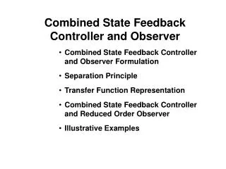
Separation Principle Plant: State Feedback Law using estimated state: State Equation: (8.6) Observer: Error Dynamics: (8.7) Modern Control Systems
Separation Principle (Cont.) From (8.6) and (8.7), we obtain the overall state equation (8.8) Eigenvalues of the overall state equation (7.17) (8.9) Equation (8.9) tells us that the eigenvalues of the observer-based state feedback system is consisted of eigenvalues of (A-BF) and (A-LC). Hence, the design of state feedback and observer gain can be done independently. Modern Control Systems
Observer-Based Control System Plant: Observer: State Feedback Law: Modern Control Systems
C B A L C B A K Fig. Observer-based control system Modern Control Systems
C B A L C B A K Fig. Observer-based control system with compensating gain Modern Control Systems
Reduced-Order Observer Design Consider the n-dimensional dynamical equation (8.10a) (8.10b) Here we assume that C has full rank, that is, rank C =q. Then, there exists a coordinate transformation which can be partitioned as (8.11) Modern Control Systems
, we have Since (8.12a) (8.12b) which become (8.13a) Plant: (8.13b) where Observer: Observer Modern Control Systems
Note that and w are function of known signals u and y. Now if the dynamical equation above is observable, an estimator of can be constructed. Theorem: The pair {A, C} in (8.10) or, equivalently, the pair in (8.12) is observable if and only if the pair in (8.13) is observable. Modern Control Systems
Let the estimate of be Such that the eigenvalues of can be arbitrarily assigned by a proper choices of . The substitution of w and into (8.143) yields (8.14) (8.15) To eliminate the term of the derivative of y, by defining (8.16) Modern Control Systems
is an estimate of . Using (8.15), then the derivative of (8.16) becomes From (8.15), we see that Define the following matrices Modern Control Systems
Reduced-Order Observer: where Modern Control Systems
C B A + + Fig. Reduced-Order Observer Modern Control Systems
Define Error Variable then we have Modern Control Systems
Since the eigenvalues of can be arbitrarily assigned, the rate of e(t) approaching zero or, equivalently, the rate of approaching can be determined by the designer. Now we combine with to form Then from We get Modern Control Systems
How to transform state equation to the form of (8.11) Consider the n-dimensional dynamical equation (8.17a) (8.17b) Here we assume that C has full rank, that is, rank C =q. Define where R is any (n-q)n real constant matrix so that P is nonsingular. Modern Control Systems
Compute the inverse of P as where Q1and Q2are nq and n(n-q) matrices. Hence, we have Modern Control Systems
Now we transform (8.17) into (8.11), by the equivalence transformation which can be partitioned as Modern Control Systems
SISO State Space System Integral Control: Augmented Plant: Modern Control Systems
State Feedback Control Design with Integrator Closed-Loop System: Modern Control Systems
Block diagram of the integral control system C B A K Fig.Block diagram of the integral control system Modern Control Systems
Example Spec. for Step Response: Percent Overshoot 10%, Settling time 0.5 sec. State Feedback Design: Modern Control Systems
From the steady state analysis in Sec. 3.4 Modern Control Systems
State Feedback Design with Error Integrator: Closed-Loop System: (8.18) Modern Control Systems
From (8.18), we get the char. eq. of the closed-loop system is (8.19) The desired char. eq. of the closed-loop system is (8.20) By comparing coefficients on left hand sides of (8.19) and (8.20), we obtain Modern Control Systems
Closed-Loop System: Final Value Theorem Steady State Error Modern Control Systems