Combined State Feedback Controller and Observer
Combined State Feedback Controller and Observer. Combined State Feedback Controller and Observer Formulation Separation Principle Transfer Function Representation Combined State Feedback Controller and Reduced Order Observer Illustrative Examples. Motivation.

Combined State Feedback Controller and Observer
E N D
Presentation Transcript
Combined State Feedback Controller and Observer • Combined State Feedback Controller and Observer Formulation • Separation Principle • Transfer Function Representation • Combined State Feedback Controller and Reduced Order Observer • Illustrative Examples
Motivation • In most control applications all state variables are not measurable • A full or reduced order observer may be used to estimate needed states • Separation principle allows independent controller and observer design
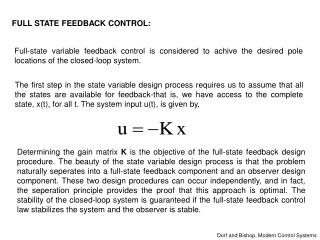
Combined Controller-Observer Formulation Plant: Controller: Observer:
State Feedback Observer Block Diagram u y r System L x y z-1 C H Observer G -K
Closed-Loop System Closed-Loop Control Subsystem: Closed-Loop Observer Subsystem: Overall Closed-Loop System:
Separation Principle Eigenvalues of the closed loop systems are the union of eigenvalues of • Closed-loop poles, i.e., eigenvalues of G-HK and • Observer poles GA-LC
Separation Principle--Transfer Function Closed-Loop System Laplace Transform: Closed-loop transfer function • Closed-loop transfer function is the same as full state feedback • Observer dynamics are canceled
Laplace Domain Representation Plant: Controller: Observer: Laplace Transform of Observer Controller in z-domain:
Transfer Function Block Digaram Representation Control Input: Solving for U gives where Y R G F1 F2
D.C. Motor Example Consider a d.c. servomotor system given by the transfer function y: position output u: input voltage the motor. Motor parameters: k/J=1 and b/J=5.
Feedback Control Design for D.C. Motor Example Desired Closed-Loop System: damping ratio =0.8 and natural frequency n=500 rad/sec (less than 3% maximum overshoot and settling time of 0.01 sec.): System in Controllable Form: Control gain
Servo Example Observer Design Observer Dynamics (2 times faster than controller): =0.8 and n=1000 rad/sec Observer gain: Observer State Equations
Equivalent Transfer Function of Servo Example Feedback and Feedforward Block: where
Closed-Loop Transfer Function R G F1 F2 Pole-zero Cancellation
Combined Controller Reduced Order Observer (CCRO) Plant State Equation: Reduced Order Observer
Transfer Function Representation of CCRO Partition State Feedback Gain: Reduced Order Observer Transfer Function Substitute Z in Control Law: where
Transfer Function Block Digaram Representation of CCRO Y R G F1 F2 F1 and F2 are of order n-q (lower than FOO)
Matlab Solution %Simulation Example of Combined Observer %System: G(s)=b/(s^2+bs) % Observable form: dx1/dt=x2, dx2/dt=-ax2+bu %System Matrices b=1; a=5; A=[0 1;0 -a]; B=[0;b]; C=[1 0]; D=0; plant=ss(A,B,C,D);
MATLAB Example Control Design %Control Design %desired closed-loop damping and natural frequency zeta=0.8; wn=500; pd=-zeta*wn+sqrt(zeta^2-1)*wn; %desired closed-loop poles %Ackermans's formula to find gain K=acker(A,B,[pd;conj(pd)]);
MATLAB Example FOO Design %Full-order observer r=2; pdo=-r*zeta*wn+r*sqrt(zeta^2-1)*wn; %desired observer poles L=(acker(A',C',[pdo;conj(pdo)]))'; Ao=A-L*C; ff=ss(Ao,B,K,0); %Part of feedforward block fb=ss(Ao,L,K,0); %Feedback Block g=-(K/Ao)*L;
MATLAB Example ROO Design %Reduced-order observer pr=-r*wn; A11=A(1,1); A12=A(1,2); B1=B(1); A21=A(2,1); A22=A(2,2); B2=B(2); K1=K(1); K2=K(2); Lr=(A22-pr)/A12; Ar=A22-Lr*A12; By=A21-Lr*A11+Ar*Lr; Bu=B2-Lr*B1; ffr=ss(Ar,Bu,K2,0); fbr=ss(Ar,By,K2,K1+K2*Lr); gr=-(K2/Ar)*By+K1+K2*Lr;
Simulation Parameters Slow Observers: r=0.5, Fast Observers: r=5 Mismatch: b=1.5 Random input and measurement noise
Slow Observer Plots FOO,ROO
Fast Observer Plots FOO,ROO
Comments on Simulation Results • Slow ROO performs better than slow FOO • High speed ROO and FOO are similar
End of Lecture 18 Next Lecture: Optimal Control