Download
1 / 57
570 likes | 688 Vues
Exercises 1: Execute step-by-step the R code at http://folk.uio.no/trondr/nve_course_3/hoelen1.R Take a look at the yearly discharge means at Hølen. This code should give answers to the following:

E N D
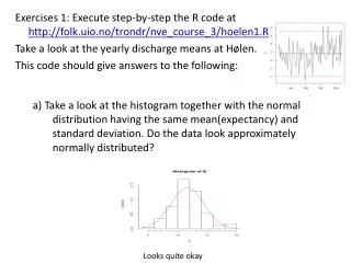
Exercises 1: Execute step-by-step the R code at http://folk.uio.no/trondr/nve_course_3/hoelen1.R Take a look at the yearly discharge means at Hølen. This code should give answers to the following: a) Take a look at the histogram together with the normal distribution having the same mean(expectancy) and standard deviation. Do the data look approximately normally distributed? Looks quite okay
Exercise 1: contd. b) Make a QQ plot to further investigate whether the data is approximately normally distributed. Also looks ok.
Exercise 1: contd. c) Do a and b over again, but this time using the lognormal distribution. (Use the mean and standard deviations of the logarithmic values to adapt the lognormal distribution to the data). Also looks ok, but not quite so good for low values (there are values that are extremely low according to the lognormal distribution). d) Repeat a-c for daily discharges also (found at http://folk.uio.no/trondr/nve_course_3/TrendDognHoelen.txt). What conclusions change and why? Extremely bad! Better but not good Yearly means are means of a large number of discharges, so the central limit theorem comes partially to the rescue. Not so for daily discharges.
Exercise 2: Is the expectancy of the yearly mean discharges at Hølen equal to 10m3/s? http://folk.uio.no/trondr/nve_course_3/hoelen2.R a) Estimate the expectancy: 11.67041 b) Check the assumption expectancy=10m3/s using a t-test (takes the variance uncertainty into account). Use preferrably a significance level of 5% (confidence level of 95%). t = 5.4363, df = 84, p-value = 5.233e-07 alternative hypothesis: true mean is not equal to 10 95 percent confidence interval: 11.05937 12.28145 sample estimates: mean of x 11.67041 95% conf. int. from 11.06 to 12.28 does not contain 10, i.e. we can reject the assumption expectancy=10 with 95% confidence. P value=0.5ppm, so we could put more confidence on this also if we wanted.
Exercise 2 condt. c) Show the data together with the confidence interval. Should we worry that most of the data is outside this interval? No. The confidence interval indicates our ucnertainty concerning the overall expectancy (long-term mean), not out uncertainty concerning single outcomes. Is it 95% probability that the real expectancy lies within this specific interval? No (trick question). A 95% confidence interval is a method that before the data has a 95% probability of encompassing the true value, whatever that value is. When you plug in the data, there is nothing more that can be assigned a probability. Frequentist methods do not have a concept about the probability concerning parameters. It’s the estimators as function of the data (when it has not yet arrived and thus has a probability) that has a probability. Once you plug data into estimators, you rather say you have a confidence regarding it
Exercise 2 contd. d) Would we be justified in using the techniques in a-c for daily data also? Exercise a could be performed and would give an unbiased estimate of the expectancy. The analysis in exercise b-c depends on independence assumptions that are not at all valid for daily data! e) Do the same analysis using the lognormal distribution also. Perform a bootstrap analysis in order to make a 95% confidence interval. What does this say about the assumption expectancy=10m3/s? The estimated 95% confidence interval does not encompass 10. (It must be told that the way to get a 95% confidence interval from bootstrap samples is a little bit naive here, to keep things simple). The confidence interval is quite similar to the one we got from the t test (i.e. under normal assumptions). Conklusjon: expectancy=10m3/s doesn’t seem to be the case.
Extra exercise 2: Outcome of dice throws On a cubic die, there is a 1/6th probability for each outcome from 1 to 6. When you have two dice, let’s assume the outcomes on the two dice are independent. a) What is the probability for a specific outcome on the two dice, for instance the probability of getting 5 on the first die and 2 on the second die? Independent outcomes: Pr(5 on the first die and 2 one the second die) = Pr(5 on the first die)*Pr(2 on the second die) = 1/6*1/6 = 1/36 b) What is the probability of getting sum=2 one the two dice? Repeat for sum=3, sum=4, sum=5, sum=6 , sum=7, sum=8. Sum=2. One way of getting this; 1-1. I.e. Pr(sum=2)=1/36 Sum=3. Two ways of getting this; 1-2, 2-1. Thus P(sum=3)=Pr(1-2)+Pr(2-1)=2/36=1/18 Sum=4. Three ways of getting this; 1-3, 2-2, 3-1. Thus Pr(sum=4)=1/36+1/36+1/36=3/36=1/12 Sum=5. Five ways of getting this; 1-4, 2-3, 3-2, 4-1. Thus Pr(sum=5)=4/36=1/9 Sum=6. Five ways; 1-5, 2-4, 3-3, 4-2, 5-1. Pr(sum=6)=5/36 Sum=7. Six ways; 1-6, 2-5, 3-4, 4-3, 5-2, 6-1. Pr(sum=7)=6/36=1/6 Sum=8. Five ways; 2-6, 3-5, 4-4, 5-3, 6-2. Pr(sum=8)=5/36
Extra exercise 2 (contd): Outcome of dice throws c) What is the probability for sum<=4? Pr(sum<=4) = Pr(sum=2 or sum=3 or sum=4) = Pr(sum=2)+Pr(sum=3)+Pr(sum=4) = 1/36+2/36+3/36=6/36=1/6 or Pr(sum<=4)=Pr(1-1)+Pr(1-2)+Pr(1-4)+Pr(2-1)+Pr(2-2)+Pr(3-1)=6/36=1/6 d) What is the probability for equal outcome on the two dice? Six different outcomes with equal dice: 1-1, 2-2, 3-3, 4-4, 5-5, 6-6 Pr(two equal)=Pr(1-1)+Pr(2-2)+…+Pr(6-6)=6/36=1/6
Extra exercise 2 (condt): Outcome of dice throws e) What is the probability of getting equal outcomes and sum<=4? Pr(two equal dice and sum<=4) = Pr(1-1)+Pr(2-2)=2/36=1/18 f) What is the probability for either getting sum<=4 or two equal dice? You can use the answers from c, d and e or you can count the possibilities. 1). Pr(two equal dice or sum<=4) = Pr(two equal)+Pr(sum<=4)-Pr(two equal and sum<=4) = 1/6+1/6-1/18 = 5/18 2). Pr(two equal or sum<=4)= Pr(1-1)+Pr(1-2)+Pr(2-1)+Pr(2-2)+Pr(1-3)+Pr(3-1)+Pr(3-3)+Pr(4-4)+Pr(5-5)+ Pr(6-6) = 10/36=5/18
Extra exercise 2 (condt): Outcome of dice throws g) Both from the rule for conditional probability and from the list of ourcomes where sum<=4, what is the probability of equal dice given that sum<=4 1). Pr(two equal | sum<=4)= Pr(two equal and sum<=4)/Pr(sum<=4)= (1/18) / (1/6) = 1/3 2). List of outcomes where sum<=4: 1-1, 1-2, 1-3, 2-1, 2-2, 3-1 Six different (equally probable) outcomes where sum<=4. (see exercise c). Two outcomes with two equal and sum<=4: 1-1 and 2-2. Therefore Pr(two equal | sum<=4)=2/6=1/3 h) Calculate the probability from sum<=4 given two equal dice, both from a list of possible outcomes and from Bayes formula. 1). List of outcomes with two equal: 1-1, 2-2, 3-3, 4-4, 5-5, 6-6. Six outcomes with equal probability. Two of these has sum<=4. Ergo Pr(sum<=4 | two equal)=1/3 2). Bayesformel:
Extra exercise 3: At Blindern, there is a 33.9% chance of rain any given day, given that it rained yesterday. There is a 12.9% chance of rain given that it didn’t rain the previous day. PS: Assume stationarity, that is that all probabilities do not depend of which day it is, when the circumstances are the same. • What is the probability that it rains any given day? (I.e. what is the marginal probability for rain?) Tip.... Pr(rain today)= Pr(rain today and rain yesterday)+Pr(rain today but not yesterday)= Pr(rain today | rain yesterday)*Pr(rain yesterday) + Pr(rain today | no rain yesterday)*Pr(no rain yesterday) = 33.9%*Pr(rain yesterday)+12.9%*(1-Pr(rain yesterday)= (stationarity) 33.9%*Pr(rain today)+12.9%*(1-Pr(rain today) Pr(rain today)*(100%-33.9%+12.9%)=12.9% ) Pr(rain today)=12.9%/79%=16.3%
Extra exercise 3 (contd): At Blindern, there is a 33.9% chance of rain any given day, given that it rained yesterday. There is a 12.9% chance of rain given that it didn’t rain the previous day. PS: Assume stationarity, that is that all probabilities do not depend of which day it is, when the circumstances are the same. b) Why is the chance of rain yesterday given that it rained today also 33.9% (Tip: Bayes formula) (stationarity)
Extra exercise 4 – conditioonal probabilities The Hobbit Shire council has decided to expand the hobbit settlements westwards. Unfortunately, these lands are infested with dragons! Of the 10kmx10km areas studied so far, 70% av were dragon-infisted. A standard protocol for examining and area was made. A standardized test area of lesser size is examined, where a field hobbit biologist goes through the area in detail. The Shire Biology Institute has determined that there is a 50% chance of detecting a dragon in an area with this procedure, if there is a dragon in that area. If there is no dragon in the area, there is of course no probability of detecting one either! Hobbit Dragon No dragons Here be dragons ? ?
Extraexercise4 contd. What is the (marginal) probability of detecting a dragon, when you don’t know whether the area is infected or not? (Hint: The law of total probability) eller The lawof total probability: Pr(detecting a dragon)=Pr(detecting a dragon | dragon in the area)*Pr(dragon in the area) + Pr(detecting a dragon | no dragon in the area)*Pr(no dragon in the area) = 50%*70%+0%*30% = 35%
Extraexercise4 contd. Dragon in the area No dragon Dragon detected Dragon detected and in the area Show using Bayes formula that the probability of there being a dragon in the area if you actually detected one, is 100%. Find the probability of there being a dragon in the area given that you did not detect one. Could you have expected the probability to decrease even without knowing the detection rate? Dragon in the area Dragon in the area No dragon No dragon Dragon detected Last question: Yes. Seegraphicalrepresentation or useevidencerulesofcourse 2.
Exercise 3: Analysis of repeat period for a given threshold value in continuous time. Will look at the danger for the discharge to go above a fixed threshold. The station Gryta has discharge>1.5m3/s 27(=y) times in the course of t=44 years. Assume such events to be independent in time, i.e. a Poisson process. Instead of rate, we will use the expected repeat period, T=1/ (where is the rate). When one has data over a time period, t, the probability for y events will then be (Poisson distribution): Show that the ML estimate is At the same time, calculate the information matrix, I(T).
Exercise 3 (contd): The likelihood is maximal at . a) What is the ML-estimate for T in this particular case? 44years/27=1.63years. b) 95% confidence interval. Sd(T)=1/I(T)=T3/2/ t=t/y3/2=0.31years. 1.63years+/-1.96*0.31years = (1.01years,2.24years).
Exercise 4: Independence, Markov chains and precipitation at Blindern Want to test whether thresholded precipitation (rain or no rain) is time dependent or not. The alternative model is a Markov chain. The rain state (0 or 1) is called xi, where i denotes the day index. Since we need to condition on the previous state, we set aside the first day, x0. The number of days except this, is denoted n. Zero hypothesis: The rain status (0 or 1) is independent from day to day (Bernoilli process). We can thus specify the model with one parameter, p=probability for rain a given day. The probability for a series of data is then: where k=number of days with rain. This will thus be the likelihood-function of this model. The ML estimate of p is then Alternative hypothesis: The rain status (0 or 1) is a Markov chain. There is a transition probability from no rain to rain pNR and a transition probability for rain given rain the previous day also, pRR. (The two other probabilities are given as the negation of the two that have been specified). The probability of a given dataset is then: where kR and nRis the number of rainy days and total days when it rained the previous day and kN and nN are similarly defined for cases where it didn’t rain the previous day. The ML estimate for the two parameters then become: pRR R 1-pRR pNR N 1-pNR
Exercise 4: Independence, Markov chains and precipitation at Blindern (contd). Check if the rain status at Blindern is time dependent or not. Code: http://folk.uio.no/trondr/nve_course_3/blindern.R. Data: http://folk.uio.no/trondr/nve_course_3/blindern_terkslet.txt. a) For the Blindern data, what is the estimate for p (rain probability in the zero hypothesis) and pNR and pRR (alternative hypothesis). From the last, what seems to be the nature of the rain status one day and the next? p=16.3% (zero hypothesis) , pNR=12.9% ogpRR=33.9% (alternative hypothesis). Rain one seems to increase the probability of rain the next day quite a bit, but not so much as to make rain more likely than no rain, it seems. b) p’=16.3% (a little difference in the further digits). c) 2*(la-l0)=138. 2(0.95)=3.84 => rejecting the zero hypothesis with 95% confidence. P value=7.6*10-32. In other words, no, the rains tate is not independent from day to day! d) 95% confidence interval for pRR: (30.1%,37.7%) 95% confidence interval for pRR: (11.7%,14.1%) e) For p, theoretic: (15.1%, 17.5%) For p, bootstrapped: (15.1%, 17.5%) For p’, bootstrapped: (14.8%, 17.8%) . It makes sense that p’ is more uncertain, since it comes from a model with more parameters and since this model suggests dependent data (thus less independent information). pRR R 1-pRR pNR N 1-pNR
Exercise 5: Medical example translated to the language of Bayesian statistics. (PS: probabilities instead of probability densities and sums instead of integrals). Reminder: 0.1% of the population has a certain sickness. There is a test that always tests positive when the subject has the sickness and only tests positive 1% of the time when the subject is healthy. a) Identify what is data outcomes and what is the thing we want to do inference on (the parameter, if you like). Data = test outcome (positive or negative test) Parameter = Sickness status (sick or healthy) b) What is the prior distribution? The prior is pre-knowledge concerning the parameter, i.e. the sickness status. Our prior knowledge is that P(sickness)=0.1%. Pr(healthy)=99.9%. c) What is the likelihood? Pr(test outcome|sickness status), giving a total of 4 combinations: Pr(positive test | sick)=100% Pr(positive test | healthy)=1% Pr(negative test | sick)=0% Pr(negative test | healthy)=99% d) Describe and calculate (using the law of total probability) the prior prediction distribution (marginal data distribution): The prior predictive distribution will here be Pr(test outcome) unconditioned on the sickness status. Pr(positive test)=Pr(positive test | sick)Pr(sick)+Pr(positive test | healthy)Pr(healthy)= 100%*0.1%+1%*99.9%=1.099% P(neg)=P(neg|sick)P(sick)+P(neg|healthy)P(healthy)=0%*0.1%+99%*99.9%=98.901%. Alt: P(neg)=100%-P(pos))=98.901%.
Exercise 5: Medical example translated to the language of Bayesian statistics. (PS: probabilities instead of probability densities and sums instead of integrals). Reminder: 0.1% of the population has a certain sickness. There is a test that always tests positive when the subject has the sickness and only tests positive 1% of the time when the subject is healthy. d) What is the posterior distribution, given a positive or a negative test? Positive test: Pr(sick|pos)=Pr(pos|sick)Pr(sick)/Pr(pos)=100%*0.1%/1.099%=9.099% Pr(healthy|pos)=100%-Pr(sick|pos)=90.9% Negative test: Pr(sick|neg)=Pr(neg|sick)Pr(sick)/P(neg)=0% P(healthy|neg)=100%-P(sick|neg)=100%
Exercise 5: Medical example translated to the language of Bayesian statistics. (PS: probabilities instead of probability densities and sums instead of integrals). Reminder: 0.1% of the population has a certain sickness. There is a test that always tests positive when the subject has the sickness and only tests positive 1% of the time when the subject is healthy. f) A little risk analysis: The cost (C) for society (patient time as well as medical staff and equipement) of a medical operation is 10000kr. The benefit (B) is 100000kr if the subject has the sickness and 0kr if not. Assume you have tested positive. Find the expected benefit (=-risk): E(B-C|positive test). If you test positive, will the oepration pay off in total? C=10.000kr, B=100.000kr if sick, B=0kr if healthy. E(B-C|pos)=(B-C|syk)Pr(sick|pos)+(B-C|healthy)Pr(healthy|pos)= (B|sick)*Pr(sick|pos)-C= 100.000kr*Pr(sick|pos)-C=100.000kr*9.099%-10.000kr= -901kr. Thus an operation now does not pay off (in expectancy). g) Assume the first test to be positive. What is the posterior prediction distribution for a new test, now? Pr(new pos|pos)=Pr(new pos|sick,pos)*Pr(sick|pos)+Pr(new pos|healthy,pos)* Pr(healthy|pos)=100%*9.099%+1%*90.9%=10.001% Pr(new neg|pos)=1-Pr(new pos|pos)=90% g) A new test is performed and again gives a positive outcome. What is now the posterior probability that you have the sickness? Will an operation now pay off in expectancy? Pr(sick|new pos, pos)=Pr(new pos | sick,pos)P(sick|pos)/P(new pos|pos)=100%*9.099%/10.001%=90.9% E(B-C|nypos,pos)=(B|sick)*Pr(sick|newpos,pos)-K=100.000kr*90.9%-10.000kr=80.917kr Now an operation will pay off!
Exercise 6: Expectation value for mean discharge at Hølen – Bayesian analysis http://folk.uio.no/trondr/nve_course_3/hoelen3.R Assume that the data is normally distributed, Then the overall mean will also be normally distributed (this will approximately be the case even if the data itself is not normally distributed). We have a vague normal prior for the data expectancy, : where 0==10. Assume we know that the standard deviation of the individual values is =2.83. a) What are the expectancy and standard deviation of the posterior distribution of in this case? Can you from this give an estimate of the data expectancy, ? If so, is that estimate far from the estimate you got from exercise 2? 11.669 now (11.670 in exercise 2). Not a big difference. b) Make a 95% credibility band for the discharge expectancy. (Tip: 95% of the probability of a normal distribution is less than 1.96 standard deviations from the expectancy). Was this much different from the 95% confidence interval in exercise 2? Can you from this conclude concerning the assumption =10m3/s? Now, 11.07-12.27, before 11.06-12.28. Not a big difference (That the interval was a little wider for the t test is reasonable, since we did not assume we knew =2.83 there). Strictly speaking you can’t conclude anything concerning the assumption =10m3/s. It’s not the most probable value, but there is no one-to-one relationship between model testing and uncertainty intervals, as there is in frequentist methodology. mu.D [1] 11.66884 tau.D [1] 0.3068121 c(mu.D-1.96*tau.D,mu.D+1.96*tau.D) [1] 11.06749 12.27019
Exercise6 – contd. The prior predictive (marginal) distribution is: c) We will now test the assumption =10. Compare the prior predictive distribution under our model (free-ranging ), with the prior predictive distribution when =10 (see the expression for the likelihood). What does this suggest? d1 = prior predictivedistributiondensity under free-ranging. d0 = prior predictivedistributiondensitywhen=10. d1>>d0 suggest thatwe have evidence for ourfree-rangingmodelratherthan for themodel=10. > d1=dnorm(mean(Q),mu.0,sqrt(tau^2+sigma^2/n)) > d1 [1] 0.03932351 > > # Probabilitydensitywhen mu=10 > d0=dnorm(mean(Q),10,sigma/sqrt(n)) > d0 [1] 4.822864e-07
Exercise 6 – contd. d) Calculate the posterior model probability for model 0 (=10) and model 1 (free-ranging ). Assume the prior model probability for each model to be 50%. What is the conclusion? 99.9988% probability for model 1 (free-ranging ) vsmodell 0 ( =10). Very probable that 10, in other words. > p0.D=d0*p0/(d0*p0+d1*p1) > p1.D=d1*p1/(d0*p0+d1*p1) > c(p0.D,p1.D) [1] 1.226443e-05 9.999877e-01
Exercise 6 – contd. e) Make a plot of the prior predictive distribution given different data outcomes and compare that to model 0. What data outcomes (if any) would be evidence for model 0, i.e. for =10? If we got a data mean between 9.19 and 10.81, the prior predictive probability density is larger for model 0 than for model 1. Thus such an outcome would be evidence for model 0 ( =10) rather than for model 1 (free-ranging ). > c(min(x[d0>d1]),max(x[d0>d1])) [1] 9.19 10.81
Exercise 7: Bayesian analysis of repeat period for a given threshold value in continuous time. Will look at the danger for the discharge to go above a fixed threshold. The station Gryta has discharge>1.5m3/s y=27 times in the course of t=44 years. Assume such events to be independent in time, i.e. a Poisson process. Instead of rate, we will use the expected repeat period, T=1/ (where is the rate). When one has data over a time period, t, the probability for y events will then be (Poisson distribution): Assume an inverse gamma distribution (which is mathematically convendient) for the parameter, T: The prior predictive (marginal) data distribution is then: (this is the so-called negative binomial distribution).
Exercise 7 (contd.): The station Gryta has had discharge>1.5m3/s y=27 times in the course of t=44 years. • Plot the prior distribution for T and the prior predictive data distribution while using ==1 in the prior. The prior has a peak around T=1, but is fairly wise. So is the prior predictive distribution. y=27 is not a particularly expectational outcome according to this model.
Exercise 7 (contd.): The station Gryta has had discharge>1.5m3/s y=27 times in the course of t=44 years. b) Use Bayes formula to express the posterior distribution for T.
Exercise 7 (contd): The station Gryta has had discharge>1.5m3/s y=27 times in the course of t=44 years. b) Use Bayes formula to express the posterior distribution for T. Plot this for Gryta when ==1. Compare to the prior distribution. Try also ==0.5 and even ==0 (non-informative) . Were there large differences in the posterior probability distribution? Compare these results with the frequentist result: TML=t/y=1.63 years. A peak (modus) is found around 1,55 years, relatively near the ML estimate. Expectation /( -1)=1.67years, median=1.63years, which is even closer. Posterior with prior Posterior using different priors Zoomet version
Exercise 7 (contd): The station Gryta has had discharge>1.5m3/s y=27 times in the course of t=44 years. c) Find the 95% credibility interval by calculating the 2.5% and 97.5% quantile of the posterior distribution, when the prior is specified by ==1. (R-tip: The 2.5% quantilen of the inverse gamma distribution is one over the 97.5% quantile of the gamma distribution and vice versa.) Compare with the 95% confidence interval in the frequentist analysis. 95% credibility interval when ==1 is used. Result: (1.15, 2.42) Asymptotic classic 95% confidence: (1.01,2.24). Not very different, though the Bayesian analysis suggest that T has a skewed distribution, so higher values are more reasonable.
Exercise 7 (contd.): d) Can you find the posterior prediction distribution for new floods at Gryta the next 100 years? If so, plot that. Compare to the Poisson distribution with the ML estimate inserted. Why is that distribution sharper than the Bayesian posterior prediction distribution? Since the posterior distribution for T comes form the same family of distributions as the prior distribution, we can just replace with *=+y and with *= +t in the predictive distribution. The Poisson distribution with a fixed parameter T is sharper than the posterior prediction distribution Simply because we do not know the exact value for T. Thus T has a distribution rather than a fixed value. Using the ML estimate doesn’t take the parameter uncertainty into account.
Exercise 7 (contd.): e) Do a simple MCMC run to fetch samples from the posterior distribution for T. Find how many samples are need before the process stabilizes (burn-in) and approximately how many samples are need before you get independent sample (spacing). Burn-in=20-40, spacing=10
Exercise 7 (contd.) f) Fetch 1000 approximately independent samples after burn-in. Compare this result with the theoretical posterior distribution (histogram and QQ plot). Looks good in my run. g) Perform an new MCMC sampling, this time with the prior distribution f(T)=lognormal(=0,=2). (This cannot be solved analytically). Compare with the samples you got in f. Pretty much the same, but maybe a few deviations in the upper tail? Relatively independent
Extra exercise 5: Extreme value analysis at Bulken (about 120 years of data). Code: http://folk.uio.no/trondr/nve_course_3/bulken_extreme.R Data: : http://folk.uio.no/trondr/nve_course_3/bulken_max.txt Will use the Gumbel distribution as model for the yearly extreme values (floods): • Make an extreme value plot, by ordering the yearly maximal discharges and plot them against expected repeat time interval where n=number of years and i is an index running from 1 to n b) Fit the Gumbel distribution to the data using the two first l-moments (see the code), 1and 2. (Extra: Compare with what you get from DAGUT). The parameters relate to the l-moments as = 2/log(2), = 1-0.57721. Calculate 1 and 2 and as DAGUT: Same result, essentially… Sorteddata > c(mu.lmom, beta.lmom) [1] 305.22055 67.96247
Extra exercise 5 – contd. c) Make an extreme value plot (extreme value against repetition time) given the l-moment estimates together with the data. Looks ok. d) Do numerical ML estimation of the parameters. e) Make an extreme value plot given the ML estimates. Fairly much the same as the l-moment estimate for small values. Slight Disagreement for larger values. > c(mu.ml, beta.ml) [1] 304.49483 74.13713
Extra extercise 5 – contd. f) (PS: If this seems mystic, stop here.) Perform a Bayesian analysis with flat prior. Sample 1000 MCMC samples (burn-in=1000, spacing=10). Compare estimated parameters with previous results. Look at the uncertainty of the parameters .Also look at the MCMC samples themselves. Has the chain of samples stabilized (is the burn-in long enough) and are the dependencies in the samples (spacing). Peaks found around mu=305, beta=75 (modus estimate). Not to different from other estimates. The histogram suggest that mu is somewhere between 290 and 320 and that the posterior distribution is approximately normal. # Expectation estimate:: > c(mean(mu.mcmc),mean(beta.mcmc)) [1] 304.81509 74.86763 # Median estimate: > c(median(mu.mcmc),median(beta.mcmc)) [1] 305.16144 74.93275
Extra exercise 5 – contd. g) Use also the posterior prediction distribution to make an extreme value plot (with the parameter uncertainty taken into account). Compare with previous results. Fairly much the same as the ML estimate.
Exercise8: Perform a power-law regression on discharge as a function of stage at station gryta, that is do a linear regression of log(discharge) against log(stage). Code: http://folk.uio.no/trondr/nve_course_3/gryta.R • Plot the data, both on the original scale and on log-scale. Seems like the points are curving upwards. Looks fairly linear
Coefficients: Estimate Std. Error t value Pr(>|t|) (Intercept) 0.93691 0.03870 24.21 2.74e-16 *** lh 2.53572 0.03841 66.03 < 2e-16 *** --- Signif. codes: 0 ‘***’ 0.001 ‘**’ 0.01 ‘*’ 0.05 ‘.’ 0.1 ‘ ’ 1 Residual standard error: 0.0492 on 20 degrees of freedom Multiple R-squared: 0.9954, Adjusted R-squared: 0.9952 F-statistic: 4359 on 1 and 20 DF, p-value: < 2.2e-16 Exercise 8 - contd b) Run a linear regression on log(discharge) against log(stage). Interpret the result. Is there a significant relationship between stage and discharge? Stage is significant, p-value<2*10^-16. R2=99.54%. Good fit. c) What is the formula for discharge vs stage on the original scale? Plot this. Q(h)=exp(0.937)*h2.536 Plot this: Looks good
Exercise 8 - contd. d) Check if anything is wrong with the residuals (trend or non-normality). No visible trend. Suggestions of a heavy upper tail, but that’s it. e) Extra: Perform a linear regression on the original scale and make a plot of this also. (PS: R code not included). Not a big success…
Exercise 9: The dataset http://folk.uio.no/trondr/nve_course_3/Env-Eco.csv contains species counts in various lakes together with some environmental variables, namely height, substrate diameter, water velocity, dissolved oxygen and water temperature. We want to see if the species richness is connected to any of the environmental variables according to this dataset. A species count can range from 0 but does not have an upper limit. Thus we will use Poisson regression (glm(family=poisson()) in R). The model looks like this: where yi is the response (number of species) for site number i and xj,i is covariate number j, site number i. Will log-transform the covariates diameter, velocityand dissolved oxygen, since these are strictly positive of nature. Code: http://folk.uio.no/trondr/nve_course_3/env_eco.R • Fetch the data and take a glance at it. .... ok • Run a Poisson fit with only a constant term (no covariates). Compare the result with the mean species number. # Compare species mean with result # from regression: > exp(3.0377) [1] 20.85722 > mean(env.eco$species.number) [1] 20.85714 glm(formula = species.number ~ 1, family = poisson(), data = env.eco) Deviance Residuals: Min 1Q Median 3Q Max -3.2221 -0.8728 -0.4149 0.6673 3.0022 Coefficients: Estimate Std. Error z value Pr(>|z|) (Intercept) 3.03770 0.05852 51.91 <2e-16 *** --- Signif. codes: 0 ‘***’ 0.001 ‘**’ 0.01 ‘*’ 0.05 ‘.’ 0.1 ‘ ’ 1 (Dispersion parameter for poisson family taken to be 1) Null deviance: 35.513 on 13 degrees of freedom Residual deviance: 35.513 on 13 degrees of freedom AIC: 105 Number of Fisher Scoring iterations: 4 Estimate Pretty much the same…
Exercise 9 – contd: c) Try each covariate in term. Are any statistically significant (according to the score test reported for each individual covariate)? If so, which is most significant (has the lowest p-value)? We have now started a stepwise-up approach to model building. Estimate Std. Error z value Pr(>|z|) height 0.0000847 0.0001283 0.66 0.509 log(diameter) 0.05215 0.03479 1.499 0.134 log(depth) -0.09970 0.09059 -1.101 0.271 log(velocity) 0.07223 0.05012 1.441 0.15 log(dissolved.oxygen) 1.450256 0.476236 3.045 0.00232 ** water.temperature -0.000748 0.0120500 -0.062 0.95 Only dissolved oxygen is statistically significant (p value < 5%) all on it’s own. d) Use the best covariate and then use that as a basis to see if there are any more significant variables (significance level 5%). If so add the most significant and see if any more can be added. If not, stop there. What does the resulting model say? Estimate Std. Error z value Pr(>|z|) height 3.852e-06 1.347e-04 0.029 0.97718 log(diameter) 0.05213 0.03604 1.446 0.1481 log(depth) -0.11330 0.09501 -1.192 0.23309 log(velocity) 0.03894 0.05306 0.734 0.46297 water.temperature -0.001036 0.011768 -0.088 0.92985 No more statistically significant covariates. Stop here. Only dissolved oxygen seems to matter. The more the merrier (species-wise).
Exercise 9 - contd: e) Now start with a large model containing all possible covariates. If any covariates are not significant, remove the most insignificant and start over again. What model do you end up with now? If there are any differences between the results now and for the stepwise-up approach, why do you think that happened? Full model: height most insignificant (highest p-value) Diameter, depth, velocity, oxygen, temperature: temperature most insignificant Diameter, depth, velocity, oxygen: velocity most insignificant Diameter, depth, oxygen: No more insignificant covariates! Result: Estimate Std. Error z value Pr(>|z|) (Intercept) 0.75258 1.13125 0.665 0.5059 log(diameter) 0.09564 0.04306 2.221 0.0263 * log(depth) -0.25871 0.11335 -2.283 0.0225 * log(velocity) 0.05423 0.05536 0.980 0.3273 log(dissolved.oxygen) 1.30535 0.49974 2.612 0.0090 ** Depth has negative impact on species richness, while substrate diameter has a positive influence, it seems. The reason why we didn’t arrive at this model when going stepwise-up might be because (log) diameter and depth are also positively correlated, correlation=47%. Thus if only one covariate , say diameter, is added then the effect will be that it gets a regression f actor 0.096 directly from the change in diameter but also a factor 0.47*(-0.26)) from the depth, since increasing diameter means increasing depth on average. The result in an effect too small to be detectable.
Exercise 10: Perform a power-law regression on discharge as a function of stage at station Gryta, that is do a linear regression of log(discharge) against log(stage-zero plane), now with unknown zero-plane. I.e. do regression on the model Code: http://folk.uio.no/trondr/nve_course_3/gryta2.R • Perform a linear regression of log-discharge on log(stage-h0) for a set of candidate values for h0. Look at the likelihood as a function of these candidate values. What is the best estimate for h0? What is the estimate for a, b, C and ? ML estimate: h0=0.08 h0[l==max(l)] [1] 0.08 c(a,b,exp(a),sigma) [1] 0.87241912 1.96226749 2.39269207 0.04131054
Exercise 10 - contd: b) A test called the likelihood-ratio test says that the zero-hypothesis is rejected with 95% confidence when 2(lfull-l0)>3.84 (PS: for one parameter). Test if h0=0. 2*(l.a-l.0) [1] 7.690884 2(la-l0)>3.84 Reject h0=0 with 95% confidence.
Extraexercise 6: Will de-trend daily data from Hølen using linear regression. Then a relatively naive ARMA time series analysis will be performed. Code: http://folk.uio.no/trondr/nve_course_3/hoelen_arima.R a) Plot thedata b) De-trend the data using linear regression on time+trigonometricfunctions over time (to catch the seasonality). Doesn’tlook like we have removed time-dependency…
ACF Extra exercise 6 - contd. c) Take a look at the residuals (i.e. the de-trended data). Is there auto-correlations there? Can we trust model selection using linear regression here? Auto-correlation: Yes! Can we trust the model selection? No! Severely aut-correlated residuals. d) Take a look at the partial auto-correlation also. Would an AR- or MA-model be expected to perform best? PACF terms die out rapidely. Seems like AR(2) might perform well, but will do things step-wise. e) Fit an AR(1) model (PS: pacf suggests AR(2) is better). Check whether the estimated parameter is approximately the same as the first term in the autocorrelation? AR(1) c oefficient=0.9472, pretty much equal to the first value in the pacf and acf plots. PACF Coefficients: ar1 intercept 0.9472 0.0000 s.e. 0.0018 0.0252
Extra exercise 6 - contd. e) Make analytic plots of the AR(1) residuals. What does these suggest? Suggests that a lot of the time dependencies have been explained, but that there is still some residual time dependency in the data. f) Also use an ARMA(1,1) model. Take another look at the residuals. What do they seem to say now? That this looks good?
Extraexercise 7: BUse the Kalman filter to interpolate over holes at the station Farstad, year 1993. Will use the simplest type of continuous time Markov chain, namely the Wiener process (random walk). The data has varying time resolution and will be log transformed before use. The system (updating) equation is: The observation equation is: In total, only two parameters, and . a) Plot thedata. Make artifical holes: 1993-02-01 00:00:00 - 1993-02-03 00:00:00 1993-03-01 12:00:00 - 1993-03-15 12:00:00 1993-08-01 00:00:00 - 1993-08-01 18:00:00 1993-09-01 00:00:00 - 1993-09-02 00:00:00 1993-10-01 00:00:00 - 1993-11-01 00:00:00 Plot the data in the holes together with the rest of the data.