Chapter 5 Cellular Concept
Chapter 5 Cellular Concept. 曾志成 國立宜蘭大學 電機工程學系 tsengcc@niu.edu.tw. R. R. Cell. R. R. (a) Ideal cell. (b) Actual cell. (c) Different cell models. Cell Shape. A cell is the radio coverage by a transmitting station or a BS. Why hexagon? closer to a circle

Chapter 5 Cellular Concept
E N D
Presentation Transcript
Chapter 5Cellular Concept 曾志成 國立宜蘭大學 電機工程學系 tsengcc@niu.edu.tw EE of NIU
R R Cell R R (a) Ideal cell (b) Actual cell (c) Different cell models Cell Shape • A cell is the radio coverage by a transmitting station or a BS. • Why hexagon? • closer to a circle • can be arranged next to each other without having any overlap and uncovered space in between R EE of NIU
Impact of Cell Shape and Radius on Service Characteristics EE of NIU
Cell i Cell j -60 -60 -70 -70 -80 -80 -90 -90 -100 -100 Select cell j on right of boundary Signal Strength Signal strength (in dBm) Select cell i on left of boundary Ideal boundary EE of NIU
Actual Signal Strength Signal strength (in dBm) Cell j Cell i -60 -70 -60 -80 -70 -90 -80 -90 -100 -100 Signal strength contours indicating actual cell tiling. This happens because of terrain, presence of obstacles and signal attenuation in the atmosphere. EE of NIU
Variation of Received Power Received power P(x) Distance x of MSfrom BS EE of NIU
Handoff Region • By looking at the variation of signal strength from either base station, it is possible to decide on the optimum area where handoff can take place. Signal strength due to BSi Signal strength due to BSj Pj(x) Pi(x) E E Pmin BSj MS BSi X1 X3 X5 Xth X4 X2 EE of NIU
R2 R1 Handoff Rate in a Rectangular Area • N1 is the number of MSs having handoff per unit length in horizontal direction • N2 is the number of MSs having handoff per unit length in vertical direction • Since handoff can occur at sides R1 and R2 of a cell N2 N1 • Assuming area A=R1R2 is fixed, substitute R2= A/R1, differentiating lH with respect to R1and equating to 0 gives N1cosq + N2sinq-A/R12 (N1sinq +N2cosq)=0 EE of NIU
Handoff Rate in a Rectangular • Thus, we have: • Simplifying through few steps gives • H is minimized when = 0, giving EE of NIU
The Offered Traffic Load of A Cell • Average number of MSs requesting service (Average arrival rate): • Average length of time MS requires service (Average holding time): T • Offered load: a =T • Example: • In a cell with 100 MSs, on an average 30 requests are generated during an hour, with average holding time T=360 seconds. Then, arrival rate =30/3600 requests/sec • A channel kept busy for an hour is defined as one Erlang EE of NIU
Analyses of The Call Blocking Probability (1) • Average arrival rate is • Average service (departure) rate is • The system can be analyzed by a M/M/S/S queuing model, where S is the number of channels • The steady state probability P(i) for this system in the form (for i=0, 1,……,S) where and EE of NIU
Analyses of The Call Blocking Probability (2) • The probability P(S) of an arriving call being blocked is the probability that all S channels are busy • This is Erlang B formula B(S, a) • Example: If S=2 and a=3, the blocking probability B(2, 3) is • So, the number of blocked calls is about 300.529=15.87 EE of NIU
The Probability of A Call Being Delayed • The efficiency of a system can be given by • The probability of a call being delayed • This is Erlang C Formula • For S=5, a=3, B(5,3)=0.11, we have C(5,3)=0.2360 EE of NIU
Erlang B and Erlang C • Probability of an arriving call being blocked is where S is the number of channels in a group. • Probability of an arriving call being delayed is where a is the traffic load in Erlang and S is the number of channels. Erlang B formula Erlang C formula EE of NIU
Frequency Reuse: 7 Cell Reuse Cluster F7 F2 F7 F2 F3 F6 F1 F3 F6 F1 F1 F5 F4 F7 F2 F5 F4 F7 F2 F1 F3 F6 F3 F6 F1 F5 F4 F5 F4 Fx: A set of frequency bands EE of NIU
Reuse Distance (1) Cluster R • For hexagonal cells, the reuse distance is given by where R is cell radius and N is the reuse pattern (the cluster size or the number of cells per cluster). • Reuse factor is F7 F2 F3 F6 F1 F5 F4 F7 F2 F3 F6 F1 F5 F4 Reuse distance D EE of NIU
60° j direction 1 2 3 … i Reuse Distance (2) • The cluster size or the number of cells per cluster is given by where i and j are integers and N = 1, 3, 4, 7, 9, 12, 13, 16, 19, 21, 28, …, etc. • The popular values of N are 4 and 7. • Finding the center of an adjacent cluster using integers i and j i direction EE of NIU
How to Form a Cluster? v (u =0) • Select a cell and make the center of the cell as the origin. • u-axis and v-axis intersects at 60-degree angle. • Define the unit distance as the distance of centers of two adjacent cells. • Each cell can then get an ordered pair (u,v) to mark the position. (-3, 3) u (v =0) 3 2 4 3 1 2 1 0 -1 -1 -2 -3 -2 -4 -3 (4, -3) EE of NIU
v u 4 2 0 5 6 3 1 5 4 2 3 6 1 6 1 2 0 5 3 4 2 0 5 3 4 1 3 6 4 0 1 2 5 1 6 4 0 3 2 4 2 0 5 1 3 6 5 6 0 1 2 3 2 3 6 4 5 1 0 6 1 2 0 5 4 4 2 0 3 5 6 1 0 3 1 6 4 5 3 1 6 4 5 0 2 4 2 0 5 3 6 6 2 0 5 4 1 3 4 3 2 1 6 5 1 3 6 4 2 0 5 Labeling Cells with L Values for N=7 (i.e. i=2, j=1) • For j=1, the cluster size is given by N=i2+i+1. • Define L=[(i+1)u+v)] mod N, we can obtain cell labels L for the cell whose center is at (u,v). • For N=7, i=2 and j=1 An alternative choice for 7-cell cluster EE of NIU
v u 5 12 9 3 10 4 11 1 8 7 12 0 6 4 8 2 3 9 10 11 11 5 12 6 0 7 9 10 7 8 2 1 3 11 6 10 4 5 12 2 9 0 1 6 7 8 5 9 3 10 11 4 1 8 5 12 7 6 0 4 10 8 2 3 9 0 12 6 7 4 11 5 9 3 8 2 7 1 4 11 5 12 6 3 10 8 7 1 2 0 6 11 5 3 10 4 9 2 7 5 12 6 0 1 8 3 10 4 2 9 1 Labeling Cells with L Values for N=13 (i.e. i=3, j=1) EE of NIU
Worst Case of Cochannel Interference (Omnidirectional Antenna) D6 R D5 D1 Mobile Station D4 D2 D3 Serving Base Station Co-channel Base Station EE of NIU
Cochannel Interference Ratio (CCIR) • Cochannel interference ratio is given by • Ik is co-channel interference from the kth co-channel interfering cell. • M is the maximum number of co-channel interfering cells • Techniques to reduce CCIR • Cell splitting • Cell sectoring EE of NIU
Cell Splitting • Depending on traffic patterns, the smaller cells may be activated/deactivated in order to efficiently use cell resources. • Smaller cell size, smaller transmitting power, and reduces cochannel interference Large cell (low traffic density) Small cell (high traffic density) Smaller cell (higher traffic density) EE of NIU
c 120o b a (c). 120o sector (alternate) f d e 60o a 90o a c d b b c (e). 60o sector (d). 90o sector Cell Sectoring by Antenna Design c 120o a b (b). 120o sector (a). Omni EE of NIU
Worst Case for Forward Channel Interference in Three-sectors BS • The CCIR in the worst case for 3-sectors • is the propagation path loss slope and = 2 ~ 5 D BS D’ MS R BS D BS EE of NIU
Worst Case for Forward Channel Interference in Six-sectors • The CCIR in the worst case for 6-sectors • is the propagation path loss slope and = 2 ~ 5 MS BS R D+0.7R BS EE of NIU
B C X A Cell Sectoring by Placing Directional Antennas at Three Common Corners EE of NIU
Homework • P5.3 • P5.4 • P5.9 • P5.10 • P5.12 • P5.19 EE of NIU