Understanding Support Vector Machines: Optimal Linear Separators and Kernel Functions
This overview of Support Vector Machines (SVMs) revisits the concept of linear classification, addressing the importance of optimal linear separators in feature space. It examines the classification margin and the role of support vectors, differentiating between hard and soft margin classifications to handle non-linearly separable data. The "kernel trick" allows for mapping data into higher-dimensional spaces to find separable features. Examples of kernel functions including linear, polynomial, and Gaussian are presented, along with practical applications of SVMs in various fields.

Understanding Support Vector Machines: Optimal Linear Separators and Kernel Functions
E N D
Presentation Transcript
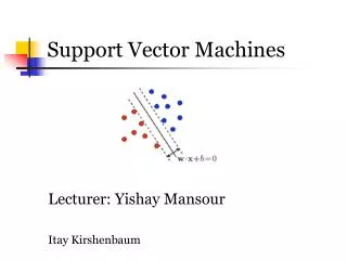
Perceptron Revisited: Linear Separators • Binary classification can be viewed as the task of separating classes in feature space: wTx + b = 0 wTx + b > 0 wTx + b < 0 f(x) = sign(wTx + b)
Linear Separators • Which of the linear separators is optimal?
Classification Margin • Distance from example xi to the separator is • Examples closest to the hyperplane are support vectors. • Marginρof the separator is the distance between support vectors. ρ r
Maximum Margin Classification • Maximizing the margin is good according to intuition and PAC theory. • Implies that only support vectors matter; other training examples are ignorable.
Soft Margin Classification • What if the training set is not linearly separable? • Slack variablesξican be added to allow misclassification of difficult or noisy examples, resulting margin called soft. ξi ξi
Linear SVMs: Overview • The classifier is a separating hyperplane. • Most “important” training points are support vectors; they define the hyperplane. • Quadratic optimization algorithms can identify which training points xiare support vectors with non-zero Lagrangian multipliers αi. • Both in the dual formulation of the problem and in the solution training points appear only inside inner products: f(x) = ΣαiyixiTx + b Find α1…αNsuch that Q(α) =Σαi- ½ΣΣαiαjyiyjxiTxjis maximized and (1)Σαiyi= 0 (2) 0 ≤αi≤ C for all αi
Non-linear SVMs • Datasets that are linearly separable with some noise work out great: • But what are we going to do if the dataset is just too hard? • How about… mapping data to a higher-dimensional space: x 0 x 0 x2 x 0
Non-linear SVMs: Feature spaces • General idea: the original feature space can always be mapped to some higher-dimensional feature space where the training set is separable: Φ: x→φ(x)
The “Kernel Trick” • The linear classifier relies on inner product between vectors K(xi,xj)=xiTxj • If every datapoint is mapped into high-dimensional space via some transformation Φ: x→φ(x), the inner product becomes: K(xi,xj)= φ(xi)Tφ(xj) • A kernel function is a function that is eqiuvalent to an inner product in some feature space. • Example: 2-dimensional vectors x=[x1 x2]; let K(xi,xj)=(1 + xiTxj)2, Need to show that K(xi,xj)= φ(xi)Tφ(xj): K(xi,xj)=(1 + xiTxj)2,= 1+ xi12xj12 + 2 xi1xj1xi2xj2+ xi22xj22 + 2xi1xj1 + 2xi2xj2= = [1 xi12 √2 xi1xi2 xi22 √2xi1 √2xi2]T [1 xj12 √2 xj1xj2 xj22 √2xj1 √2xj2] = = φ(xi)Tφ(xj), where φ(x) = [1 x12 √2 x1x2 x22 √2x1 √2x2] • Thus, a kernel function implicitly maps data to a high-dimensional space (without the need to compute each φ(x) explicitly).
Examples of Kernel Functions • Linear: K(xi,xj)= xiTxj • Mapping Φ: x→ φ(x), where φ(x) is x itself • Polynomial of power p: K(xi,xj)= (1+xiTxj)p • Mapping Φ: x→ φ(x), where φ(x) has dimensions • Gaussian (radial-basis function): K(xi,xj) = • Mapping Φ: x→ φ(x), where φ(x) is infinite-dimensional: every point is mapped to a function (a Gaussian); combination of functions for support vectors is the separator. • Higher-dimensional space still has intrinsic dimensionality d (the mapping is not onto), but linear separators in it correspond to non-linear separators in original space.
SVM applications • SVMs were originally proposed by Boser, Guyon and Vapnik in 1992 and gained increasing popularity in late 1990s. • SVMs are currently among the best performers for a number of classification tasks ranging from text to genomic data. • SVMs can be applied to complex data types beyond feature vectors (e.g. graphs, sequences, relational data) by designing kernel functions for such data. • SVM techniques have been extended to a number of tasks such as regression [Vapnik et al. ’97], principal component analysis [Schölkopf et al. ’99], etc. • Most popular optimization algorithms for SVMs use decomposition to hill-climb over a subset of αi’s at a time, e.g. SMO [Platt ’99] and [Joachims ’99] • Tuning SVMs remains a black art: selecting a specific kernel and parameters is usually done in a try-and-see manner.

