Download
1 / 48
510 likes | 904 Vues
5.5 Graphs of Other Trigonometric Functions. Objectives: Understand the graph of y = sin x . Graph variations of y = sin x . Understand the graph of y = cos x . Graph variations of y = cos x . Use vertical shifts of sine and cosine curves.

E N D
5.5 Graphs of Other Trigonometric Functions • Objectives: • Understand the graph of y = sin x. • Graph variations of y = sin x. • Understand the graph of y = cosx. • Graph variations of y = cosx. • Use vertical shifts of sine and cosine curves. • Model periodic behavior. Dr .Hayk Melikyan Department of Mathematics and CS melikyan@nccu.edu
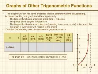
Some Properties of the Graph of y = sinx The domain is The range is [–1, 1]. The function is an odd function: The period is
Example: Graphing a Variation of y = sinx • Determine the amplitude of Then graph • and for • Step 1 Identify the amplitude and the period. • The equation is of the form y = Asinx with A = 3. Thus, the amplitude is This means that the maximum value of y is 3 and the minimum value of y is – 3. The period is
Example: Graphing a Variation of y = sinx (continued) • Determine the amplitude of Then graph • and for • Step 2 Find the values of x for the five key points. To generate x-values for each of the five key points, we begin by dividing the period, by 4. The cycle begins at x1 = 0. We add quarter periods to generate x-values for each of the key points.
Example: Graphing a Variation of y = sinx (continued) • Step 3 Find the values of y for the five key points.
Example: Graphing a Variation of y = sinx (continued) • Determine the amplitude of Then graph • and for • Step 4 Connect the five key • points with a smooth curve • and graph one complete cycle • of the given function. amplitude = 3 period
Example: Graphing a Function of the Form y = AsinBx • Determine the amplitude and period of Then graph the function for • Step 1 Identify the amplitude and the period. • The equation is of the form y = A sinBx with A = 2 and • The maximum value of y is 2, the minimum value of y is –2. The period of tells us that the graph completes one cycle from 0 to period: amplitude:
Example: Graphing a Function of the Form y = AsinBx (continued) • Step 2 Find the values of x for the five key points. • To generate x-values for each of the five key points, we begin by dividing the period, by 4. The cycle begins at x1 = 0. We add quarter periods to generate x-values for each of the key points.
Example: Graphing a Function of the Form y = AsinBx (continued) • Step 3 Find the values of y for the five key points.
Example: Graphing a Function of the Form y = AsinBx (continued) • Determine the amplitude and period of Then graph the function for • Step 4 Connect the five key points • with a smooth curve and graph • one complete cycle of the • given function. amplitude = 2 period
Example: Graphing a Function of the Form y = AsinBx (continued) • Determine the amplitude and period of Then graph the function for • Step 5 Extend the graph in step 4 to the left or right as desired. We will extend the graph to include • the interval amplitude = 2 period
Example: Graphing a Function of the Form y = Asin(Bx – C) • Determine the amplitude, period, and phase shift of • Then graph one period of the function. • Step 1 Identify the amplitude, the period, and the phase shift. period: amplitude: phase shift:
Example: Graphing a Function of the Form y = Asin(Bx – C) (continued) • Step 2 Find the values of x for the five key points.
Example: Graphing a Function of the Form y = Asin(Bx – C) (continued) • Step 3 Find the values of y for the five key points.
Example: Graphing a Function of the Form y = Asin(Bx – C) (continued) • Step 3 (cont) Find the values of y for the five key points.
Example: Graphing a Function of the Form y = Asin(Bx – C) (continued) • Step 4 Connect the five key points with a smooth curve and graph one complete cycle of the function amplitude = 3 phase shift period
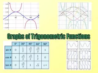
Some Properties of the Graph of y = cosx The domain is The range is [–1, 1]. The function is an even function: The period is
Sinusoidal Graphs The graphs of sine functions and cosine functions are called sinusoidal graphs. The graph of is the graph of with a phase shift of
Example: Graphing a Function of the Form y = AcosBx • Determine the amplitude and period of • Then graph the function for • Step 1 Identify the amplitude and the period. period: amplitude:
Example: Graphing a Function of the Form y = AcosBx (continued) • Determine the amplitude and period of • Then graph the function for • Step 2 Find the values of x for the five key points.
Example: Graphing a Function of the Form y = AcosBx (continued) • Step 3 Find the values of y for the five key points.
Example: Graphing a Function of the Form y = AcosBx (continued) • Step 3 Find the values of y for the five key points.
Example: Graphing a Function of the Form y = AcosBx (continued) • Determine the amplitude and period of • Then graph the function for • Step 4 Connect the five key • points with a smooth curve • and graph one complete • cycle of the given function. amplitude = 4 period = 2
Example: Graphing a Function of the Form y = AcosBx (continued) • Determine the amplitude and period of • Then graph the function for • Step 5 Extend the graph • to the left or right • as desired. amplitude = 4 period = 2
Example: Graphing a Function of the Form y = Acos(Bx – C) • Determine the amplitude, period, and phase shift of • Then graph one period of the function. • Step 1 Identify the amplitude, the period, and the phase shift. amplitude: period: phase shift:
Example: Graphing a Function of the Form y = Acos(Bx – C) (continued) • Determine the amplitude, period, and phase shift of • Then graph one period of the function. • Step 2 Find the x-values for the five key points.
Example: Graphing a Function of the Form y = Acos(Bx – C) (continued) • Step 3 Find the values of y for the five key points.
Example: Graphing a Function of the Form y = Acos(Bx – C) (continued) • Step 3 (cont) Find the values of y for the five key points.
Example: Graphing a Function of the Form y = Acos(Bx – C) (continued) • Step 3 (cont) Find the values of y for the five key points.
Example: Graphing a Function of the Form y = Acos(Bx – C) (continued) • Determine the amplitude, period, and phase shift of • Then graph one period of the function. • Step 4 Connect the five • key points with • a smooth curve • and graph one • complete cycle of the • given function. amplitude period
Vertical Shifts of Sinusoidal Graphs • For sinusoidal graphs of the form • and • the constant D causes a vertical shift in the graph. • These vertical shifts result in sinusoidal graphs oscillating about the horizontal line y = D rather than about the x-axis. • The maximum value of y is • The minimum value of y is
Example: A Vertical Shift • Graph one period of the function • Step 1 Identify the amplitude, period, phase shift, and vertical shift. period: amplitude: one unit upward vertical shift: phase shift:
Example: A Vertical Shift • Graph one period of the function • Step 2 Find the values of x for the five key points.
Example: A Vertical Shift • Step 3 Find the values of y for the five key points.
Example: A Vertical Shift • Step 3 (cont) Find the values of y for the five key points.
Example: A Vertical Shift • Graph one period of the function • Step 4 Connect the five • key points with • a smooth curve • and graph one • complete cycle of • the given function.
Example: Modeling Periodic Behavior • A region that is 30° north of the Equator averages a minimum of 10 hours of daylight in December. Hours of daylight are at a maximum of 14 hours in June. Let x represent the month of the year, with 1 for January, 2 for February, 3 for March, and 12 for December. If y represents the number of hours of daylight in month x, use a sine function of the form y = Asin(Bx – C) + D to model the hours of daylight. • Because the hours of daylight range from a minimum of 10 to a maximum of 14, the curve oscillates about the middle value, 12 hours. Thus, D = 12.
Example: Modeling Periodic Behavior(continued) • A region that is 30° north of the Equator averages a minimum of 10 hours of daylight in December. Hours of daylight are at a maximum of 14 hours in June. Let x represent the month of the year, with 1 for January, 2 for February, 3 for March, and 12 for December. If y represents the number of hours of daylight in month x, use a sine function of the form y = Asin(Bx – C) + D to model the hours of daylight. • The maximum number of hours of daylight is 14, which is 2 hours more than 12 hours. Thus, A, the amplitude, is 2; A = 2.
Example: Modeling Periodic Behavior • A region that is 30° north of the Equator averages a minimum of 10 hours of daylight in December. Hours of daylight are at a maximum of 14 hours in June. Let x represent the month of the year, with 1 for January, 2 for February, 3 for March, and 12 for December. If y represents the number of hours of daylight in month x, use a sine function of the form y = Asin(Bx – C) + D to model the hours of daylight. • One complete cycle occurs over a period of 12 months.
Example: Modeling Periodic Behavior • The starting point of the cycle is March, x = 3. • The phase shift is
Example: Modeling Periodic Behavior • A region that is 30° north of the Equator averages a minimum of 10 hours of daylight in December. Hours of daylight are at a maximum of 14 hours in June. Let x represent the month of the year, with 1 for January, 2 for February, 3 for March, and 12 for December. If y represents the number of hours of daylight in month x, use a sine function of the form y = Asin(Bx – C) + D to model the hours of daylight. The equation that models the hours of daylight is