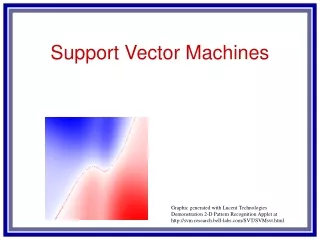
Support Vector Machines
Support Vector Machines. Stefano Cavuoti 11/27/2008. SVM.

Support Vector Machines
E N D
Presentation Transcript
SupportVectorMachines Stefano Cavuoti 11/27/2008
SVM Supportvectormachines (SVM) are a group of supervised learning methods that can be applied to classification or regression. In a short period of time, SVM found numerousapplicationsin a lotofscientificbrancheslikephysics, biology, chemistry. • drug design (discriminating between ligands and nonligands, inhibitors and noninhibitors, etc.), • quantitative structure-activity relationships (QSAR, where SVM regression is used to predict various physical, chemical, or biological properties), • chemometrics (optimization of chromatographic separation or compound concentration prediction fromspectral data asexamples), • sensors(for qualitative and quantitative prediction from sensor data), • chemical engineering (fault detection and modeling of industrial processes), • text mining (automatic recognition of scientificinformation) • etc.
SVM Classification SVM models were originally defined for the classification of linearly separableclassesofobjects. For any particular set of two-class objects, an SVM finds the unique hyperplanehaving the maximum margin. H3 (green) doesn't separate the 2 classes. H1 (blue) does, with a small margin and H2 (red) with the maximum margin.
SVM Classification The hyperplaneH1 defines the border with class +1 objects, whereas the hyperplane H2 defines the border with class 1 objects. Two objects from class +1 define the hyperplane H1, and three objects from class -1 define the hyperplane H2. These objects, represented inside circles in Figure, are called support vectors. A special characteristic of SVM is that the solution to a classification problem is represented by the support vectors that determine the maximummarginhyperplane.
SVM Classification In a plane, combinations of three points from two classes can be separated with a line. Four points cannot be separated with a linear classifier. SVM can also be used to separate classes that cannot be separated with a linear classifier. In such cases, the coordinates of the objects are mapped into a feature space using nonlinear functions called feature functions ϕ. The feature space is a high-dimensional space in which the two classes can be separated with a linear classifier.
SVM Classification The nonlinear feature function ϕ combines the input space (the original coordinates of the objects) into the feature space, which can even have an infinite dimension. Because the feature space is high dimensional, it is not practical to use directly feature functions ϕ in computing the classification hyperplane. Instead, the nonlinear mapping induced by the feature functions is computed with special functions called kernels. Kernels have the advantage of operating in the input space, where the solution of the classification problem is a weighted sum of kernel functions evaluated at the support vectors. The implementation of SVM we use has 4 kernels:
SVM- TOY Thisis a simpletoydevelopedby the creatorsof LIBSVM: Chih-Wei Hsu, Chih-Chung Chang, and Chih-Jen Lin in order ofillustrate a simple case, itisnice.
SVM Classification To illustrate the SVM capability of training nonlinear classifiers, consider the patterns fromTable. This is a synthetic dataset of two-dimensional patterns, designed to investigate the properties of the SVM classification method. In all figures, class +1 patterns are represented by + , whereas class -1 patterns are represented by black dots. The SVM hyperplane is drawn with a continuous line, whereas the margins of the SVM hyperplane are represented by dotted lines. Support vectors from the class +1 are represented as + inside a circle, whereas support vectors from the class -1 are represented as a black dot inside a circle Param 1 Param 2
SVM Classification Linear Polynomialdegree =2 Polynomialdegree = 3 Polynomialdegree = 10 RadialBasisFunction Gamma = 0.5 As we can see the linearkerneldoesn’t works in thisexample, the other 4 tests discriminate perfectly the twoclassesbutwe can seethatsolutions are quitedifferenteachother, isimportanthave a test set in ordertochoose the best one and avoid the over – fitting, the other bad news isthatkernelfunctios (except the linearone) are notproperlyfunctionsbut family offunctions so weneedtotryvariousparameters (usuallycalledHyperParameter) tomake the best choise
Selection of active of galaxies in terms of a minimal set of parameters embodying their physical differences as closely as possible (in this case, whether an AGN is contained or not). Most galaxy classifications are based on morphological informations, which only partly reflect the physical differences between different class of objects. One clear example is represented by galaxies containing AGNs, which do not fit comfortably inside any morphological classification known (except weak correlations). A data-mining approach, as machine learning methods, can be highly effective to select AGN-hosting galaxies. Classification of Active Galactic Nuclei The aim of this work is find a way to select the AGN hosting galaxies using just photometric parameters using supervised machine learning methods and a spettroscopic Base of Knowlendge (hereafter BoK)
Seyfert I: galaxies for which these relations are satisfied: (FWHM(Hα) > 1.5*FWHM([OIII] λ5007) AND FWHM([OIII] λ5007) < 800 Km s-1 OR FWHM(Hα) > 1200 Km s-1 ) Kewley’s line • Emission lines ratio catalogue (Kauffman et al, 2003) • 0.05 < z < 0.095 • Mr < -20.0 • AGN’s selected according to Kewley’s empirical method (Kewley et al. 2001): • AGN’s catalogue (Sorrentino et al, 2006) Kauffman’s line The data used for the BoK Heckman’s line Seyfert II: all remaining galaxies. The BoK is formed by objects residing in different regions of the BPT plot (Baldwin, Phillips and Tellevich 1981).
Heckman’s line The BoK Kewley’s line Kauffman’s line log(OIII)/Hβ log(NII)/Hα
Photometric redshifts catalogue based on SDSS-DR5 catalogues (D’Abrusco et al., 2007) PhotoObjAll table (SDSS-DR5) 1 0 1 1 0 0 Photometric parameters Photometric parameters used for training of the NNs and SVMs: petroR50_u, petroR50_g, petroR50_r, petroR50_i, petroR50_z concentration_index_r fibermag_r (u – g)dered, (g – r)dered, (r – i)dered, (i – z) dered dered_r photo_z_corr Target values: 1° Experiment: AGN -> 1, Mixed -> 0 2° Experiment: Type 1 -> 1, Type 2 -> 0 3° Experiment: Seyfert -> 1, LINERs -> 0
log2(γ) log2(C) SVM There are a lotofimplementationofSupportVectorMachines and a lotofmethodtodo the samethings, wechoose the mostusedimplementation, the LIBSVM implementedbyChih-Wei Hsu, Chih-Chung Chang, and Chih-Jen Lin, thatprovides 2 methodsforclassificationandtwomethodsforregression, eachmethodmayrequireoneortwootherHyper Parameters so thecrucialpointusing SVM isthetuningoftheHyper Parameter (eitherofthekerneleitherofthespecificmethod) . In mythesis I used C-SVC asmethodandradial basisfunctionaskernel, so I had an Hyper Parameter fromthekernel (gamma) and a Hyper Parameter fromthemethod (C) I usedthestrategy of the 2-dim parameter plane (gamma, C) for the SVM (proposed by Hsu, Chang et Lin) consists in running different jobs on a grid whose knots are spaced by a factor 4 on both parameters (γ = 2−15, 2−13…23, C = 2−5, 2−3, ...215). So 110 process for each classification problem, in the figure you can see a contour diagram, different colors correspond to different level of accuracy so you can see in which area the best results are confined and you may refine the tuning. Cross-validation of results and “folding” (5 subsets) of the dataset are used for all experiments. Efficiency:
Results* • Checking the trained NN with a datasetofsurenot AGN just 12.6% are false positive • False positive surelynot AGN (accordingBoK) are 0.89% AGN~55% SVM ~74% Not AGN ~87% MLP ~76% etyp1~82% Type1 ~99% SVM etyp2~86% MLP etyp2~99% Type2 ~100% etyp1~98% ~78% Seyfert~53% SVM MLP LINERs~92% ~80% ∗C., D’Abrusco, Longo, 2008, in preparation.
Ongoing work: improving AGN class. 1. Improving the accuracy of the photometric parameters deriving them directly by the images (in coll. with R. De Carvalho and F. La Barbera). The improvement of the Base of Knowledge can be accomplished not only enhancing the quality of spectroscopic classification, but also by enlarging the wavelength range whence the BoK is extracted. This is a possible approach to connect different types of AGNs. AGNs classification can be refined by: 2. Improving the effectiveness of separation between different families using better spectroscopic indicators, i.e. using a better BoK (in coll. with P. Rafanelli and S. Ciroi)