Download
1 / 95
1.06k likes | 1.81k Vues
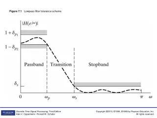
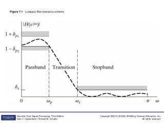
Figure 7.1 Lowpass filter tolerance scheme. Figure 7.2 Basic system for discrete-time filtering of continuous-time signals. Figure 7.3 Illustration of aliasing in the impulse invariance design technique.

E N D
Figure 7.2 Basic system for discrete-time filtering of continuous-time signals.
Figure 7.3 Illustration of aliasing in the impulse invariance design technique.
Figure 7.4s-plane locations for poles of Hc (s)Hc(−s) for 6th-order Butterworth filter in Example 7.2.
Figure 7.5 Frequency response of 6th-order Butterworth filter transformed by impulse invariance. (a) Log magnitude in dB. (b) Magnitude. (c) Group delay.
Figure 7.6 Mapping of the s-plane onto the z -plane using the bilinear transformation.
Figure 7.7 Mapping of the continuous-time frequency axis onto the discrete-time frequency axis by bilinear transformation.
Figure 7.8 Frequency warping inherent in the bilinear transformation of a continuous-time lowpass filter into a discrete-time lowpass filter. To achieve the desired discrete-time cutoff frequencies, the continuous-time cutoff frequencies must be prewarped as indicated.
Figure 7.9 Illustration of the effect of the bilinear transformation on a linearphase characteristic. (Dashed line is linear phase and solid line is phase resulting from bilinear transformation.)
Figure 7.10s-plane locations for poles of Hc(s)Hc(−s) for 6th-order Butterworth filter in Example 7.3.
Figure 7.11 Frequency response of 6th-order Butterworth filter transformed by bilinear transform. (a) Log magnitude in dB. (b) Magnitude. (c) Group delay.
Figure 7.15 Elliptic filter, 5th-order, exceeds design specifications.
Figure 7.16 Elliptic filter, 5th-order, minimizing the passband ripple.
Figure 7.17 Frequency response of 14th-order Butterworth filter in Example 7.5. (a) Log magnitude in dB. (b) Detailed plot of magnitude in passband. (c) Group delay.
Figure 7.17 (continued) (d) Pole–zero plot of 14th-order Butterworth filter in Example 7.5.
Figure 7.18 Frequency response of 8th-order Chebyshev type I filter in Example 7.5. (a) Log magnitude in dB. (b) Detailed plot of magnitude in passband. (c) Group delay.
Figure 7.19 Frequency response of 8th-order Chebyshev type II filter in Example 7.5. (a) Log magnitude in dB. (b) Detailed plot of magnitude in passband. (c) Group delay.
Figure 7.20 Pole–zero plot of 8th-order Chebyshev filters in Example 7.5. (a) Type I. (b) Type II.
Figure 7.21 Frequency response of 6th-order elliptic filter in Example 7.5. (a) Log magnitude in dB. (b) Detailed plot of magnitude in passband. (c) Group delay.
Figure 7.22 Pole–zero plot of 6th-order elliptic filter in Example 7.5.
Figure 7.24 Warping of the frequency scale in lowpass-to-lowpass transformation.
Table 7.1 TRANSFORMATIONS FROM A LOWPASS DIGITAL FILTER PROTOTYPE OF CUTOFF FREQUENCY θp TO HIGHPASS, BANDPASS, AND BANDSTOP FILTERS
Figure 7.25 Frequency response of 4th-order Chebyshev lowpass filter. (a) Log magnitude in dB. (b) Magnitude. (c) Group delay.
Figure 7.26 Frequency response of 4th-order Chebyshev highpass filter obtained by frequency transformation. (a) Log magnitude in dB. (b) Magnitude. (c) Group delay.
Figure 7.27 (a) Convolution process implied by truncation of the ideal impulse response. (b) Typical approximation resulting from windowing the ideal impulse response.
Figure 7.28 Magnitude of the Fourier transform of a rectangular window (M = 7).
Figure 7.30 Fourier transforms (log magnitude) of windows of Figure 7.29 with M = 50. (a) Rectangular. (b) Bartlett.
Figure 7.30 (continued) (c) Hann. (d) Hamming. (e) Blackman.
Figure 7.31 Illustration of type of approximation obtained at a discontinuity of the ideal frequency response.
Figure 7.32 (a) Kaiser windows for β = 0, 3, and 6 and M = 20. (b) Fourier transforms corresponding to windows in (a). (c) Fourier transforms of Kaiser windows with β = 6 and M = 10, 20, and 40.
Figure 7.33 Comparison of fixed windows with Kaiser windows in a lowpass filter design application (M = 32 and ωc= π/2). (Note that the designation “Kaiser 6” means Kaiser window with β = 6, etc.)
Figure 7.34 Response functions for the lowpass filter designed with a Kaiser window. (a) Impulse response (M = 37). (b) Log magnitude. (c) Approximation error for Ae (ejω).
Figure 7.35 Response functions for type I FIR highpass filter. (a) Impulse response (M = 24). (b) Log magnitude. (c) Approximation error for Ae (ejω).
Figure 7.36 Response functions for type II FIR highpass filter. (a) Impulse response (M = 25). (b) Log magnitude of Fourier transform. (c) Approximation error for Ae (ejω).
Figure 7.38 Response functions for type III FIR discrete-time differentiator. (a) Impulse response (M = 10). (b) Magnitude. (c) Approximation error for A0(ejω).
Figure 7.39 Response functions for type IV FIR discrete-time differentiator. (a) Impulse response (M = 5). (b) Magnitude. (c) Approximation error for A0(ejω).
Figure 7.40 Tolerance scheme and ideal response for lowpass filter.
Figure 7.41 Typical frequency response meeting the specifications of Figure 7.40.
Figure 7.42 Weighted error for the approximation of Figure 7.41.
Figure 7.43 5th-order polynomials for Example 7.8. Alternation points are indicated by ◦.
Figure 7.44 Typical example of a lowpass filter approximation that is optimal according to the alternation theorem for L = 7.
Figure 7.45 Equivalent polynomial approximation functions as a function of x = cos ω. (a) Approximating polynomial. (b) Weighting function. (c) Approximation error.
Figure 7.46 Possible optimum lowpass filter approximations for L = 7. (a) L + 3 alternations (extraripple case). (b) L + 2 alternations (extremum at ω = π). (c) L + 2 alternations (extremum at ω = 0). (d) L + 2 alternations (extremum at both ω = 0 and ω = π).