Download
1 / 41
420 likes | 584 Vues
This document outlines key concepts in pricing volatility derivatives, as presented by Bruno Dupire in 2006. It covers various models for implied and historical volatility, methods for pricing VIX futures, and the theoretical underpinnings of volatility swaps. The paper highlights the complexities of volatility sensitivity and examines the dynamics between spot prices and volatility. It also discusses the importance of log profile approaches in hedging strategies and the implications of skew and correlation in volatility products, offering a comprehensive view of the rapidly evolving landscape of derivatives trading.

E N D
Model Free Results onVolatility Derivatives Bruno Dupire Bloomberg NY SAMSI Research Triangle Park February 27, 2006
Outline • I VIX Pricing • II Models • III Lower Bound • IV Conclusion
Historical Volatility Products • Historical variance: • OTC products: • Volatility swap • Variance swap • Corridor variance swap • Options on volatility/variance • Volatility swap again • Listed Products • Futures on realized variance
Implied Volatility Products • Definition • Implied volatility: input in Black-Scholes formula to recover market price: • Old VIX: proxy for ATM implied vol • New VIX: proxy for variance swap rate • OTC products • Swaps and options • Listed products • VIX Futures contract • Volax
Vanilla Options Simple product, but complex mix of underlying and volatility: Call option has : • Sensitivity to S : Δ • Sensitivity to σ : Vega These sensitivities vary through time, spot and vol :
Volatility Games To playpure volatility games (eg bet that S&P vol goes up, no view on the S&P itself): • Need of constant sensitivity to vol; • Achieved by combining several strikes; • Ideally achieved by a log profile : (variance swaps)
Log Profile Under BS: dS = σS dW, For all S, The log profile is decomposed as: In practice, finite number of strikes CBOE definition: Put if Ki<F, Call otherwise FWD adjustment
Perfect Replication of We can buy today a PF which gives VIX2T1 at T1: buy T2 options and sell T1 options.
Theoretical Pricing of VIX Futures FVIX before launch • FVIXt: price at t of receiving at T1 . The difference between both sides depends on the variance of PF (vol vol), which is difficult to estimate.
Pricing of FVIX after launch Much less transaction costs on F than on PF (by a factor of at least 20) • Replicate PF by F instead of F by PF!
Bias estimation can be estimated by combining the historical volatilities of F and Spot VIX. Seemingly circular analysis : F is estimated through its own volatility!
VIX Summary • VIX Futures is a FWD volatility between future dates T1 and T2. • Depends on volatilities over T1 and T2. • Can be locked in by trading options maturities T1 and T2. • 2 problems : • Need to use all strikes (log profile) • Locks in , not need for convexity adjustment and dynamic hedging.
Volatility Modeling • Neuberger (90): Quadratic variation can be replicated by delta hedging Log profiles • Dupire (92): Forward variance synthesized from European options. Risk neutral dynamics of volatility to fit the implied vol term structure. Arbitrage pricing of claims on Spot and on vol • Heston (93): Parametric stochastic volatility model with quasi closed form solution • Dupire (96), Derman-Kani (97): non parametric stochastic volatility model with perfect fit to the market (HJM approach)
Volatility Modeling 2 • Matytsin (99): Parametric stochastic volatility model with jumps to price vol derivatives • Carr-Lee (03), Friz-Gatheral (04): price and hedge of vol derivatives under assumption of uncorrelated spot and vol increments • Duanmu (04): price and hedge of vol derivatives under assumption of volatility of variance swap • Dupire (04): Universal arbitrage bounds for vol derivatives under the sole assumption of continuity
Variance swap based approach(Dupire (92), Duanmu (04)) • V = QV(0,T) is replicable with a delta hedged log profile (parabola profile for absolute quadratic variation) • Delta hedge removes first order risk • Second order risk is unhedged. It gives the quadratic variation • V is tradable and is the underlying of the vol derivative, which can be hedged with a position in V • Hedge in V is dynamic and requires assumptions on
Stochastic Volatility Models • Typically model the volatility of volatility (volvol). Popular example: Heston (93) • Theoretically: gives unique price of vol derivatives (1st equation can be discarded), but does not provide a natural unique hedge • Problem: even for a market calibrated model, disconnection between volvol and real cost of hedge.
Link Skew/Volvol • A pronounced skew imposes a high spot/vol correlation and hence a high volvol if the vol is high • As will be seen later, non flat smiles impose a lower bound on the variability of the quadratic variation • High spot/vol correlation means that options on S are related to options on vol: do not discard 1st equation anymore From now on, we assume 0 interest rates, no dividends and V is the quadratic variation of the price process (not of its log anymore)
Skewvolvol To make it simple:
Carr-Lee approach • Assumes • Continuous price • Uncorrelated increments of spot and of vol • Conditionally to a path of vol, X(T) is normally distributed, (g: normal sample) • Then it is possible to recover from the risk neutral density of X(T) the risk neutral density of V • Example: • Vol claims priced by expectation and perfect hedge • Problem: strong assumption, imposes symmetric smiles not consistent with market smiles • Extensions under construction
Spot Conditioning • Claims can be on the forward quadratic variation • Extreme case: where is the instantaneous variance at T • If f is convex, Which is a quantity observable from current option prices
X(T) not normal => V not constant • Main point: departure from normality for X(T) enforces departure from constancy for V, or: smile non flat => variability of V • Carr-Lee: conditionally to a path of vol, X(T) is gaussian • Actually, in general, if X is a continuous local martingale • QV(T) = constant => X(T) is gaussian • Not: conditional to QV(T) = constant, X(T) is gaussian • Not: X(T) is gaussian => QV(T) = constant
The Main Argument • If you sell a convex claim on X and delta hedge it, the risk is mostly on excessive realized quadratic variation • Hedge: buy a Call on V! • Classical delta hedge (at a constant implied vol) gives a final PL that depends on the Gammas encountered • Perform instead a “business time” delta hedge: the payoff is replicated as long as the quadratic variation is not exhausted
Trader’s Puzzle • You know in advance that the total realized historical volatility over the quarter will be 10% • You sell a 3 month Put at 15% implied • Are you sure you can make a profit?
Answers • Naïve answer: YES Δ hedging with 10% replicates the Put at a lower cost Profit = Put(15%) - Put(10%) • Classical answer: NO Big moves close to the strike at maturity incur losses because Γ<< 0. • Correct answer: YES Adjust the Δ hedge according to realized volatility so far Profit = Put(15%) – Put(10%)
Delta Hedging • Extend f(x) to f(x,v) as the Bachelier (normal BS) price of f for start price x and variance v: with f(x,0) = f(x) • Then, • We explore various delta hedging strategies
Calendar Time Delta Hedging • Delta hedging with constant vol: P&L depends on the path of the volatility and on the path of the spot price. • Calendar time delta hedge: replication cost of • In particular, for sigma = 0, replication cost of
Business Time Delta Hedging • Delta hedging according to the quadratic variation: P&L that depends only on quadratic variation and spot price • Hence, for And the replicating cost of is finances exactly the replication of f until
Hedge with Variance Call • Start from and delta hedge f in “business time” • If V < L, you have been able to conduct the replication until T and your wealth is • If V > L, you “run out of quadratic variation” at t < T. If you then replicate f with 0 vol until T, extra cost: where • After appropriate delta hedge, dominates which has a market price
Lower Bound for Variance Call • : price of a variance call of strike L. For all f, • We maximize the RHS for, say, • We decompose f as Where if and otherwise Then, Where is the price of for variance v and is the market implied variance for strike K
Lower Bound Strategy • Maximum when f” = 2 on , 0 elsewhere • Then, (truncated parabola) and
Arbitrage Summary • If a Variance Call of strike L and maturity T is below its lower bound: • 1) at t = 0, • Buy the variance call • Sell all options with implied vol • 2) between 0 and T, • Delta hedge the options in business time • If , then carry on the hedge with 0 vol • 3) at T, sure gain
IV Conclusion • Skew denotes a correlation between price and vol, which links options on prices and on vol • Business time delta hedge links P&L to quadratic variation • We obtain a lower bound which can be seen as the real intrinsic value of the option • Uncertainty on V comes from a spot correlated component (IV) and an uncorrelated one (TV) • It is important to use a model calibrated to the whole smile, to get IV right and to hedge it properly to lock it in