Multi-Layer Perceptrons for Non-Linear Classification
E N D
Presentation Transcript
Multi-layer perceptron Usman Roshan
Non-linear classification with many hyperplanes • Least squares will solve linear classification problems like AND and OR functions but won’t solve non-linear problems like XOR
Multilayer perceptrons • Many perceptrons with hidden layer • Can solve XOR and model non-linear functions • Leads to non-convex optimization problem solved by back propagation
Solving XOR with multi-layer perceptron z1 = s(x1 – x2 - .5) z2 = s(x2 – x1 - .5) y = s(z1 + z2 - .5)
Activation functions • Without this a neural network is just another linear classifier (can you prove it?) • Some typical activations (sign not shown)
Theorems on neural networks • Any continuous function can be approximated by a single layer neural network within epsilon error (Hornik et. al. 1991)
Theorems on neural networks • An earlier result on approximation capabilities of neural networks (Cybenko 1989)
How do we optimize neural net parameters? • First let’s look at the least squares objective again • Let our datapoints xi be in a matrix form X = [x0,x1,…,xn-1] and let y = [y0,y1,…,yn-1] be the output labels. • Then the perceptron output can be viewed as wTX = yT where w is the perceptron. • And so the perceptron problem can be posed as
Multilayer perceptron • For a multilayer perceptron with one hidden layer we can think of the hidden layer as a new set of features obtained by a linear transformation of each feature. • Let our datapoints xi be in a matrix form X = [x0,x1,…,xn-1],y = [y0,y1,…,yn-1] be the output labels, and Z = [z0,z1,…,zn-1] be the new feature representation of our data. • In a single hidden layer perceptron we have perform k linear transformations W = [w1,w2,…,wk] of our data where each wi is a vector. • Thus the output of the first layer can be written as
Multilayer perceptrons • We convert the output of the hidden layer into a non-linear function. Otherwise we would only obtain another linear function (since a linear combination of linear functions is also linear) • The intermediate layer is then given a final linear transformation u to match the output labels y. In other words uTnonlinear(Z) = y’T. For example nonlinear(x)=sign(x) or nolinear(x)=sigmoid(x). • Thus the single layer objective can be written as • Regularized version would be • The back propagation algorithm solves this with gradient descent but coordinate descent can also be applied.
Gradient descent • Recall the objective from above • We differentiate this w.r.t. each weight to obtain the gradient • Alternatively we can take a stepwise approach called back-propagation. • In this method we use the chain rule to calculate partial derivatives and perform the update for each node
Back propagation • Ilustration of back propagation • http://home.agh.edu.pl/~vlsi/AI/backp_t_en/backprop.html • Derivation: https://en.wikipedia.org/wiki/Backpropagation#Intuition
Training issues for multilayer perceptrons • Adaptive learning rate • Overfitting (a big problem in neural networks)
Training issues for multilayer perceptrons • Overfitting (a big problem in neural networks) • New methods employing randomness are highly effective • Dropout (ignore weights for randomly chosen nodes during training) • Use different subsets of the input data across iterations • Data augmentation (used for images)
