RTL Level Power Optimization Techniques
Explore dynamic, static, and leakage power components with techniques like clock gating, data path optimization, and bus design. Learn about active and leakage power issues, dynamic power reduction principles, and clock gating implementation methods for efficient low-power electronics design.

RTL Level Power Optimization Techniques
E N D
Presentation Transcript
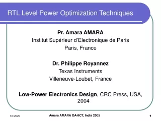
RTL Level Power Optimization Techniques Pr. Amara AMARA Institut Supérieur d’Electronique de Paris Paris, France Dr. Philippe Royannez Texas Instruments Villeneuve-Loubet, France Low-Power Electronics Design, CRC Press, USA, 2004
RTL Level Power Optimization Techniques • Introduction • Dynamic, static and leakage components • Low Power design Techniques • Clock Gating • Data paths • Buses
Hottest chips published in ISSCC 1000 x1.4 / 3 years 100 x4 / 3 years 10 Power per chip [W] 1 0.1 MPU DSP 0.01 1980 1985 1990 1995 2000 Year (Sakurai 2003)
Dynamic Power P = α CL VS VDD FCLK • The switching activity a is the average percentage of the nodes that actually toggles 0->1 in the total chip • The switching activity includes glitches spurious activity • The switching activity increases dramatically with pipelining • CL is the total equivalent Capacitance • CL includes both gate and wire capacitance • CL is an average capacitance (Caps vary with biasing, Xtalk, …)
Gate Source Drain ISTH IG+Iii N+ N+ IPT IGIDL IR P Bulk Leakage Power Issues • Pleakage : 4 dominant mechanisms • Subthreshold leakage • Gate tunneling leakage • Reverse-bias diffusion leakage • Gate-induced drain leakage (GIDL)
Active leakage may dominate 1/100 10000 Leakage Dynamic 1000 x1.4 / 3 years x1.1 / 3 years 100 ITRS requirement x4 / 3 years Power per chip [W] 10 1 0.1 MPU Processors published in ISSCC DSP 0.01 1980 1985 1990 1995 2000 2005 2010 2015 Year (Sak 2003)
Principle for Dynamic Power Reduction • Lowering switching probability (a) • Gated clock, Conditional F/F • Low transition coding • Lowering load capacitance (CL) • Embedded memory, Gate sizing • Low-k • Lowering supply voltage (VS ,VDD) • Most effective (∝VDD2) and popular, but at the cost of speed degradation • VTH should also be lowered for high-speed circuit operation • Lowering operating frequency (fCLK) • Better algorithm, parallelism • Never employed in PC, but will be important for portable devices P = α CL VS VDD FCLK
RTL Level Power Optimization Techniques • Introduction • Dynamic, static and leakage components • Low Power design Techniques • Clock Gating • Data paths • Buses
Clock Gating • Most effective power optimization technique • Supported by most of the EDA tools • Effective at register level as well as at clock network level • Different approaches: • Functional approach • Activity-driven • Observability Don’tCare-Driven
Clock Gating Principle • Goal Disable or suppress transitions from propagating to parts of the clock path (FFs, clock network and logic) under a given IDLE condition. • Principle To each sequential functional unit is associated a block CG which inhibits the clock signal when the IDLE condition is true. The IDLE condition is computed by function Fcg
Clock Gating Implementation Flip-Flop-Based Design Simplest way to implement block CG but subject to spikes. When CLK is low, spikes are filtered by the AND When CLK is high, spikes are filtered by the Latch When CLK is high, spikes are filtered by the NOR When CLK is low, spikes are filtered by the Latch
Flip-Flop-Based Design: Physical Constraint • Two separate processes in the same hierarchy • Physically Close to reduce the impact on the skew and to prevent from unwanted optimizations • Use tool specific attributes
CG : Process (CLK, CTRL) variable qint : std_logic ; begin if clk = '0' then qint := ctrl; end if; CLKG <= (not Qint) and CLK ; end process; process (CLKG) begin if CLKG = '1' then if WR ='1' then RF(conv_integer(adrA)) <= datain ; else A <= RF(conv_integer(adrA)) ; B <= RF(conv_integer(adrB)) ; end if; end if; end process ; Example
Automatic GC insertionfunctional approach • Detect conditional behavior in the VHDL description: • If then else statement, Case statement … • Identify the idle conditions (under which the clock of the element can be shut off) • Insert clock gating circuits if the user constraints are met (delay, power). • Generate modified VHDL description
P1 : process (clk) begin if clk'event and clk='1' then X <= A + B ; D <= E ; end if ; end process ; P2 : process (Gclk) begin if Gclk'event and Gclk='1' then if (load='1') then Y <= C ; end if ; end if ; end process ; P3: process (clk, load) Variable c_load: std_logic; begin if clk = '0' then c_load <= load ; end if ; Gclk <= clk and c_load ; end process ; P0 : process (clk) begin if (clk'event and clk='1') then X <= A + B; D <= E; if (load='1') then Y <= C; end if ; end if ; end process ; P1 Without CG P0 P2 with CG P3 CG circuit Example
Automatic GC insertionActivity-Driven • Most of the clock toggles are not needed • Power is wasted in the clock driver and in the register • Good candidate for Clock Gating
Automatic GC insertionActivity-Driven • Given a realistic test bench: • Sort the flips-flips according to increasing switching activity • For a predefined threshold, select a subset of low frequency flip-flops (SLF-FFs) • Locate or create an enable signal • Apply Clock Gating to the selected subset of flip-flops if the user constraints are met.
Automatic GC insertionObservability Don’t Care-Driven • If out_bus is not active during a given clock cycle, CG can be applied to R1 and R2 • An ODC boolean function is evaluated at each clock cycle to set properly the CG control signal for the next clock cycle. • This function is derived by backward traversal of the circuit using ODC method.
En 0 Out Out Q Data0 Data 1 Data Data1 En Sel CK ODC Method: Basics ODC(Data) = EN’@T-1 ODC(Data0) = Sel ODC(Data1) = Sel’ ODC(Data) = En’ (R1_en)'@T-1 + ODC(A_Bus) ((Mux_sel)' + ENB') ENB'
Automatic GC insertionODC-Driven CG Cell ODC Boolean Function R1_en R2_en Mux_sel ENB CK
Design Issues: Timing • In most power design flows: CG is inserted before clock tree synthesis • To avoid setup and/or hold time violation: • Evaluate these critical times • Set appropriate tool’s dependent variables to specify these times
Design Issues: Testability • CG introduces multiple clock domains in the design • Insert a control point (OR gate) controlled by an additional signal: Scan _mode • This signal eliminates the function of the clock gate during the test phase
Without clockgating 30.6mW DEU VDE With clock gating 8.5mW MIF DSP/ HIF 0 5 10 15 20 25 Power [mW] 896Kb SRAM How effective is Clock-gating? 90% of F/F’s were clock-gated. 70% power reduction by clock-gating alone. MPEG4 decoder M. Ohashi,Matsushita, ISSCC 2002
RTL Level Power Optimization Techniques • Introduction • Dynamic, static and leakage components • Low Power design Techniques • Clock Gating • Data paths • Buses
Data Paths • An important amount of energy may be wasted in the data path. Many techniques have been proposed: • Computational Kernel • Pre-computation logic • Guarded evaluation (operand isolation) • Control signal gating • Glitch reduction…
Computation Kernels • A sequential circuit may have a large number of reachable states. • Only a subset is visited when the circuit is in its Steady-State. • Definition: CK of a sequential circuit is a logic block that mimics the typical behavior of the original network.
Computation Kernels • IDEA: • Extract the computational Kernel (K) from the Original Circuit description (OC) • K is usually: • Small • Fast • Low Power • Realize a parallel implementation of K and OC that: • Uses K as often as possible • Uses OC otherwise
S2 S1 S0 S4 S3 S5 S2 S1 S6 S7 S1 S0 S4 S3 S0 S4 S5 Kernel S6 S7 NK Computation Kernels p1 OC p0 p4 p0, p1, p4 > pthreshold
p Comb Logic 0 FF X O Mux t 1 S r 0 S Kernel s Mux u 1 FF FF SEL Computation Kernels • SEL=1 K can compute next state and outputs • SEL=0 C must compute next state and outputs
Data Path: Pre-Computation Principle: • Partition the inputs into pre-computed and gated inputs • If output Y is independent of gated inputs then predictor G generates a signal that freezes the outputs of R2. • Function G is not unique best trade-off to find
Data Path: Guarded Evaluation • Applicable to combin. Blocks emb. within logic • If Y is idle, transparent latches are inserted to all inputs • Control circuitry is added to determine the IDLE condition • The IDLE condition is used to disable the latches.
Data Path: Control-Signal Gating • The control-signal technique takes advantage of a fine granularity analysis to reduce the switching activity in the data path buses • Principle: detect when a bus is not used and stop the propagation of the switching activity through the module(s) driving the bus • ODC-based technique Power Management Unit to generate the gated signals that control steering modules
Data Path: Control-Signal Gating (1) R1_en_gated = reg1_en AND (not(mux_sel OR (not enb)))@(T+1) R2_en_gated = reg2_en AND (not(not mux_sel OR not enb))@(T+1) (mux_sel_gated) @T = (mux_sel_gated) @(T-1) if ((not enb) @(T+1) = = True) (2) (3) The suffix @T means the value of a variable or a function at the current clock cycle, @T-1 the value one clock cycle before and finally @T+1 the value at the next clock cycle.
Data Path: Control-Signal Gating R1EG : process (Clk) begin if (Clk'Event and Clk='1') then R1_en_tmp <= NOT(mux_sel OR (NOT Enb)) ; end if ; R1_en_gated <= R1_en_tmp AND reg1_en; end process ; R2EG : process (Clk) begin if (Clk'Event and Clk='1') then R2_en_tmp<= NOT(NOT(mux_sel) OR (NOT Enb)) ; end if ; R2_en_gated <= R2_en_tmp AND reg2_en; end process ; MSG : process (Clk) begin if (Clk'Event and Clk='1') then Enb_int <= NOT Enb ; if ( Enb_int = '0' ) then mux_sel_gated <= mux_sel ; end if ; end if ; end process ; Equation 1 Equation 2 Equation 3
RTL Level Power Optimization Techniques • Introduction • Dynamic, static and leakage components • Low Power design Techniques • Clock Gating • Data paths • Buses
Bus Coding • Advanced SoC characterized by: • Long buses with high capacitance and a significant switching activity. • Techniques proposed: • Low swing bus • Charge recycling bus • Bus pipelining • Bus multiplexing • Bus encoding
b(t) Sender Receiver b(t) b(t) B(t) Receiver Sender Decoder Encoder Bus Coding Less switching activity B(t): Code word b(t): Source word
Bus Coding • Different approaches: • Bus-Invert Coding and its variants (four) • Transition Signaling Code • Offset Code • T0 Code and its variants (four) • Limited-Weight Code (ie. One-hot code) • Etc…
(b(t), 0) if H <= N/2 (B(t), INV(t)) = (b’(t), 1) Otherwise Bus Invert Coding • The encoding depends on Hamming distance between the present bus value B(t) and the next bus value B(t+1) N: number of bus lines, H: Hamming Distance
Bus Invert Coding Binary (31 Trs) BIC (19 Trs) 00101010 00111011 2 11010100 7 11110100 1 00001101 6 01110110 6 00010001 5 10000100 4 00101010 00111011 0 2 00101011 1 2 11110100 1 1 00001101 0 3 10001001 1 3 00010001 0 4 10000100 0 4
Bus Invert Coding • Characteristics: • Redundant bit consumes power • Switching activity on highly capacitive buses is reduced at the expense of additional switching activity in the decoder/encoder • Effective when the data to be transmitted is randomly distributed in time ( µP cache) • Not efficient for address bus encoding
Bus Invert Coding (Variants) • Partial BIC: • Breaks source words into 2 parts and apply BIC on one part only • Effective if certain bits of the data stream exhibit a strong spatio-temporal correlation. • Interleaving BIC: • Similar tp PBIC but partitioning and encoding are dynamically changed • M-bits BIC: • Breaks source words into M parts and encodes separately each one • Extra cost due to increasing number of INV signals
Code word B1,B2……………….Xi…………………………..Bn Bn+1 INV vector INV1,INV2……….INVi…………………….INVn Source word b1,b2……………….bi…………………………..bn bi = (Bi, INVi) Bus Invert Coding (Variants) • BIC in Time: • The decoder decodes the last n code words based on the INV vector received as the n+1 code word
T0 Code • Exploit the sequentiality of the address buses • Redundant line INC is added to the bus • When two addresses to be transmitted are sequential, the address bus is frozen and INC is set to 1 • Zero-Transition for ideally consecutive addresses
Encoder (B(t-1), 1) If b(t) = b(t-1) + S (B(t), INC(t)) (b(t), 0) Otherwise Decoder (B(t-1) + S) If INC = 1 b(t) B(t) If INC = 0 T0 Code: Principle S may be known by the encoder and the decoder or send on the bus
T0 Code: example 4 00000100 00000100 0 5 00000101 1 00000100 11 6 00000110 2 00000100 10 7 00000111 1 00000100 10 8 00001000 4 00000100 10 6 00000110 3 00000110 02 7 00000111 1 00000110 11 8 00001000 4 00000110 10 Binary encoding: T0 encoding: 16 Transitions 4 Transitions
T0 Code: Implementation Encoder Decoder
T0 Code • Suitable for address bus encoding when sequential addresses transmitted on the bus dominate. • The encoder inserts one clock cycle delay • Extra area and delay • Power saving achieved if the probability of sequential addresses appearing in the bus is higher than a technology dependent threshold
T0 Code: Variants • TO-BI Code: • Suitable when address bus is used to transmit instructions and address values • If the address are sequential, TO code is applied and the bus is frozen, otherwise the Bus Invert coding is applied Two redundant lines are necessary
Conclusions • Guidelines for power optimization at RTL level have been presented • It’s the responsibility of the designer to find the good tradeoff between power, performance areaand complexity • Tools implementing some of these techniques are available: • Synopsys • Atrenta • BullDast • Sequence Design