Low Power and Energy Optimization Techniques
Low Power and Energy Optimization Techniques. Zack Smaridge Everett Salley. 1/42. Energy-Efficient Scheduling on Heterogenous Multicore Architectures. J. Cong, B. Yuan University of California International Symposium on Low Power Electronics and Design, 2012. 2 /42. Introduction.


Low Power and Energy Optimization Techniques
E N D
Presentation Transcript
Low Power and Energy Optimization Techniques Zack Smaridge Everett Salley 1/42
Energy-Efficient Scheduling on Heterogenous Multicore Architectures J. Cong, B. Yuan University of California International Symposium on Low Power Electronics and Design, 2012 2/42
Introduction • Increase of transistors guided by Moore's Law has lead to more and more cores on a chip • On-chip power is becoming a critical issue • Intelligent scheduling may taken advantage of tradeoffs to reduce power consumption • Paper examines phase-based scheduling • Increasing use of heterogeneous multi-core architectures over homogeneous multi-core systems • Heterogeneous cores provide different power/performance trade offs 3/42
Heterogeneous Scheduling Approaches • Schemes addressing power • Sampling-based dynamic switching heuristics • Statically map program cores based on resource demands for the entire execution • Identify program phases by tracking program counters with history table • Proposed approach uses combination of static analysis and runtime scheduling • Reduces sampling overhead • Does not require large hardware additions 4/42
Energy Efficient Scheduling Scheduling Steps • Static analysis and instrumentation • Takes sources code as input • Analyze code to identify loops/loop boundaries • Calculates invocation times, number of instructions, caller-callee sites and tracks relationships • Profile program to construct call graph • Each node is a function call or loop • Infers average number of executed instructions per loop 5/42
Scheduling Steps Continued • Identify major program phases • Call graph identifies loops that qualify • Must meet minimum thresholds for instruction and invocation counts to offset overhead • Instrumentation functions inserted at the edges of identified phases • Runtime Scheduling • During each invocation two pieces of hardware data are collected • Use regression model to estimate energy consumption • Predicts EDP to make scheduling decisions 6/42
Complexity and Scalability • Complexity: O(PxN) • P – Number of major program phases • N – Number of different types of processors • Scalability becomes an issue as the number of cores increases • Use hierarchically sampling to reduce overhead • Cluster processors in to categories based on characteristics • Scheduling first determines appropriate category then maps to specific processor 7/42
Heterogeneous Multi-core Architectures • Intel QuickIA platform • Employs two asymmetric processors in terms of performance and power • Excellent platform for evaluation of heterogeneous scheduling • Intel Atom Processor 330 • Low-power microarchitecture targeted for mobil devices • Intel Xeon Processor E5450 • High performance server-class microarchitecture 8/42
Energy Efficiencies • Energy Delay Product (EDP) – measurement of power consumption per switching period • Figure 1 shows EDP for Atom vs. Xeon • SPEC Benchmark 473.astar • Each interval contains 50 million instructions • Differences in EDP for each processor depending on program phase • Potential to reduce EDP by adaptively mapping the program to the most appropriate core 9/42
EDP Measurements Figure 1: EDP on Xeon and Atom processors vs. instruction intervals for the SPEC CPU2006 Benchmark 10/42
Regression Modeling for Energy • Predicts energy usage based on training data • Data based on 4 benchmarks from SPEC CPU2006: astar, bzip2, h264ref and hmmer • Collected 15 pieces of hardware performance data for each • Data entered into McPAT to calculate energy consumption for each instruction interval • McPAT – integrated power, area and timing modeling framework that supports multicore configurations • Obtained 2000 training data samples 11/42
Hardware Performance Data Use variable clustering and correlation analysis to identify 4 key parameters: Table 1: Collected Hardware Performance Data 12/42
Predicting Energy Consumption • Linear regression model created from 4 key parameters: • Regression coefficients B determined from training data using ordinary least-squares method • Average model error: • Atom: 2.25% • Xeon: 2.6% 13/42
Regression Model Results Figure 2: Regression model can accurately predict energy consumption in a) Xeon and b) Atom processors 14/42
Evaluation Methodology • Benchmarks • SPU2006: astar, bzip2, h264ref, hmmer, lbm, libquantum and named • Medical imaging domain: denoise, deblure, registration(reg) and segmentation(seg) • Scheduling comparisons • Statical mapping approach (SMap) – statically maps programs to cores based on programs inherent characteristics. Does not switch during execution. • Periodic sampling approach (PS) – samples cores at set intervals and schedules. Modified approach is based upon pre-collected hardware performance data. 15/42
Results of Scheduling Comparison Figure 2: Normalized results of scheduling results with interval lengths of 1, 10 and 50 million instructions 16/42
Conclusion • Compared against statistical mapping • Average 10.20% reduction up to 35.25% • Did worse in 4 benchmarks: hmmer, lbm, libquantum and namd • Worse results attributed to switching overhead and application always running more efficiently on one particular core • Compared against periodic sampling • Average 19.81% reduction at 1 million instructions • Average 26.25% reduction at 10 million instructions • Average 25.31% reduction at 50 million instructions 17/42
Comparing PhaseSampAgainst PS Table 2: Comparison of EDP and core switching over benchmark sets 18/42
Future Improvements • Regression model based on only 4 benchmarks and checked against only 1 benchmark • Run time scheduling is only capable of measuring 2 pieces of hardware data at each invocation • Error rate increases sharply for less than 4 pieces of hardware performance data 19/42
Energy-Efficient Signal Processing in Wearable Embedded Systems – An Optimal Feature Selection Approach H. Ghasemzadeh, N Amini, M. Sarrafzadeh University California International Symposium on Low Power Electronics and Design, 2012 20/42
Wearable Embedded Systems Wearable Electronics are computational elements that are tightly coupled with the human body 21/42
Scope of the Paper • Classification Applications - Map physiological sensor data to specific user states • Typically achieved by extracting features from the sensor signals then applying machine learning and pattern classification algorithms 22/42
Scope of the Paper • Classification Applications - Map physiological sensor data to specific user states • Typically achieved by extracting features from the sensor signals then applying machine learning and pattern classification algorithms 23/42
Scope of the Paper • Problem – Feature extraction consumes both time and energy. Performing feature extraction on an extensive set of signals may rapidly deplete battery. • Observation – Many features may be redundant or unnecessary. Some features may be more computationally intensive to extract. • Solution – Determine the optimal set of features which minimizes power cost while still accurately classifying the data. • Introduce a new feature selection algorithm which considers the computational complexity of extracting each feature 24/42
Examples of features 25/42
Example System Sensors Sensor Node Gateway (Smartphone) Internet Sensors Sensor Node Sensors Sensor Node Data Center 26/42
Feature Selection Process • Only performed in the training phase • Construct on exhaustive set of initial features • Discard unnecessary features based on relevance and redundancy • Relevance • A feature is irrelevant if it is not useful to a specific classification application • Redundancy • A feature is redundant if it strongly correlates with other features 27/42
Proposed Selection Process New Feature Selection Process • Construct exhaustive feature set • Eliminate all irrelevant features • Perform redundancy analysis and construct a redundancy graph. Include computational complexity. • Use the graph model so solve an optimization problem 28/42
Symmetric Uncertainty U(X,Y):= Symmetric Uncertainty H(X) := Entropy of RV X I(X,Y) := Information Gain between RV X and Y • Symmetric Uncertainty is the normalized information gain and has value between 0 and 1 • U = 0 → Both RVs are completely independent • U = 1 → Knowing value of 1 RV allows you to completely predict the value of the other RV • Basically a measure of correlation between two RVs, but it also captures non-linear correlations 29/42
Relevance and Redundancy 30/42
Redundancy Graph Vertices connected by edges indicates a strong correlation between the pair of features indicates the relevant features W represents the computing cost associated with the given feature 31/42
Minimum Cost Feature Selection Goal: Find a subset of vertices in the redundancy graph that are not dominated by any other vertex (ie no redundancy) while minimizing the total cost MCFS problem is equivalent to the Minimum Cost Dominating Set (MCDS) problem which is NP-Hard Authors formulate the problem using ILP and propose a solution using Greedy Algorithms 32/42
Greedy Approach 33/42
Feature Selection Example 1 1 1 1 10 1 1 1 1 1 Total Cost = 2 Total Cost = 3 34/42
Experimental Set-up Wearable sensor with an Accelerometer and Gyroscope attached to TI MSP430 microprocessor 3 human test subjects instructed to perform 14 transitional movements Collected data was partitioned into two disjoint groups for training and testing 35/42
Results 270 51 36/42
Results 44 4 37/42
Results 47 5 38/42
Results 39/42
Conclusion ILP and Greedy approach yield very similar results Tradeoff between classification accuracy and total power savings 40/42
Future Improvements/Criticisms Dynamic feature selection – contextual info such as location or time to be used in real-time to eliminate features and deactivate unused sensor nodes No comparison to any previous works Never specify how energy savings are determined (ie 72.7% average power savings with respect to what?) 41/42
Questions? 42/42