Device Simulation: Transport (Double Gate MOSFETs)
Device Simulation: Transport (Double Gate MOSFETs). Mehdi Salmani Jelodar , Seung Hyun Park, Zhengping Jiang, Tillmann Kubis , Michael Povolotsky , Jim Fonseca, Jean Michel Sellier , Gerhard Klimeck msalmani@purdue.edu Network for Computational Nanotechnology (NCN)

Device Simulation: Transport (Double Gate MOSFETs)
E N D
Presentation Transcript
Device Simulation:Transport (Double Gate MOSFETs) MehdiSalmaniJelodar, Seung Hyun Park, Zhengping Jiang, TillmannKubis, Michael Povolotsky, Jim Fonseca, Jean Michel Sellier, Gerhard Klimeck msalmani@purdue.edu Network for Computational Nanotechnology (NCN) Electrical and Computer Engineering Purdue University Network for Computational Nanotechnology (NCN) 1
Outline • Device Modeling Approach • Device Simulation Test Samples • Device structure • Sample input decks: input parameters description • Output files and MATLAB scripts • *.VTK files: structures / charge distribution • MATLAB scripts: Extract ON-current, S.S, and DIBL from I-V characteristics • Band structure calculation and effective mass extraction
Device Modeling Approach NEMO5 Output Post Processing Input Extract Device Performance Parameters: ON-current, S.S, and DIBL m* from Full Band / Literature, Band offset, Electron affinity 2-D / 3-D NEGF (or transfer matrix) & Poisson Solver: Effective Mass Approximation Like: ID-VG characteristics, Charge distributions ION SS=60
Device Simulation Set-Up LCH LCH LD LS LD LS Gate Gate TOX SiO2 TOX SiO2 Source Si Channel Drain Source Si Channel Drain TCH SiO2 SiO2 Gate NS,D Tox (EOT) TCH LCH LS LD 1e20 cm-3 0.6nm 5nm 11nm 10nm 10nm • Simulation Features (ITRS 2020): • Channel material: Si • SiO2 as dielectric material • Channel length / thickness : 11 nm / 5nm • Doping concentration: 1e20 cm-3
Required Files on Workspace • 1. Go to: • /apps/share64/nemo/examples/current/public_examples/TransportDG/ • Subfolders: • MatlabFiles • TB2EMInputDecks • TransportInputDecks • outputs_VD005 • outputs_VD068
Device Simulation Test Samples • Read the sample input deck: ./TranportInputDecks/inputDeckMetaDG.in • Structure: • First block defines tag, material, crystal structure, and lattice size • Second block addresses effective masses (mx,my, mz), also multi-valley can be defined by using multiple delta • In third block, band gap can be modulated. • Fourth block defines doping type (N/P), and doping concentration. • Also, different region number must be assigned to each material. 3 effective masses (m*_delta1, m*_delta2 and m*_delta3) are for 6 degenerate valleys.
Device Domain • Device Domain: • In the first block, the domain name, type can be defined. • base_materialis the channel material for the central of device. • passivation_regions is for the oxide areas in case of necessary (TB usage) • In second block, dimension creates a canvas of “unit cells”, representing total dimension. • periodic sets a “false” refers to a confined axis along k direction.
Device Domain (cont.) • Device Domain: • In the first block, the coordinate system within the crystal_direction can be set up. • In space orientations first one is the first entry of periodic option. Only 2 directions need to be specified. NEMO5 computes the third using the crystal structure info. • In the second block, the starting cell coordinate is determined. • The contact and geometry description are shown in the third block. (Some output can be generated by de-commenting the output line.)
Device Domain (cont.) • Device Domain: • In the first block, the domain name, typecan be defined. • Same material is used for contacts -> base_material = channel • In the second block, the contact direction (lead_direction) can be specified. • “-1” indicates the direction of the incoming electrons. This means that n=1 for +x, n=-1 for -x, n=2 for +y, and n=-2 for –y.
Device Geometry • Device Geometry: • Each component has an order of information as shown in the below. • Firstly, base shapeof the region, and previously assigned region_numberneed to be addressed. • In min and max, the exact location and size can be adjusted. Unit is [nm] • Secondly, priority must be assigned for each component. This arranges the order of overlapping when the whole structure is built. SiO2 1 Si (source) 2 Si (channel) 2 Si (drain) 2
Device Geometry (cont.) • Device Geometry: • Top and bottom gates must be defined as same way as other components. • However, Boundary_regionmust be used as the tag for contacts instead of Region used in the other components. • The gates (min and max) are normally sandwiching the insulator (SiO2) and channel regions.
NEMO5 Meta-Solver (1) • Meta-solver: • First it determines the solver’s name and type. By type NEMO5 will look for “MetaUTBTransport.py” in . / Meta • In transport_type it can be transfer_matrixor NEGF. For EM modeling usually transfer_matrix is faster. • We need to determine transport domain, active regions, prefix of of all output files names and as many contacts we have in the device. • In the second part, the applied voltages to source, drain and gate(s) are set up.
NEMO5 Meta-Solver (2) • In first unit: • Poisson will provide the potential otherwise it will be zero. • tb_basis will determine the type of tight-binding basis should be used • Charge_self_consistant make it self-consistent with the NEGF or semi-classical (by turning on use_semiclassical_potential) • In second unit: • Number_of_enegry_points and numbe_of_momentum_points determine the number of E and K. • Momentum_intervals determines the region of calculations in Brillouin Zone. • Momentum_space_degenracydetermines the degeneracy factor (2 for degeneracy and 2 for making the k region just in positive space)
NEMO5 Meta-Solver (3) • output will provide the required output files during the simulation and some of these info will be stored in the VTK files • output_along_path and path_points and number_of_path_pointstell the simulator to dump out only information along the path with the #points precision. • enable_structure makes the structure VTK file.
Outputs with VTK files Device Schematic Insulator 6.2nm Y Channel Drain Source Y [nm] X 0nm 31nm X [nm] 0nm Electron Density [/cm2] • VTK files: • *.VTK file is created in the beginning of the simulation. • The device structure can be checked by using the VTK file in Paraview / Visit. • Charge density profile for each bias points can be obtained and checked. Off state Y [nm] On state X [nm] For regions load into visit/paraview DG2020_structure.vtk For charge density ./outputs_VD068/DG_Ramper_X.vtk
Output files and MATLAB scripts Gate ID-VG Characteristics SiO2 Y Source Si Channel Drain Si DG UTB SiO2 X 75 Gate Conduction Band edges ID [μA/μm] 5900 S.S [mv/dec] 78 DIBL [mV/V] ION[μA/μm] VGS[V] X[nm]
MATLAB scripts (1) -- > Load required files and set the variables: clear all;clc;close all; DIR1 = ‘../outputs_VD068/' DIR2 = ‘../outputs_VD005/' IVVdd = load([DIR1 ‘DG_Ramper_current.dat']); IVV05 = load([DIR2 ‘DG_Ramper_current.dat']); Vdd = 0.68; IdOff = 0.1; %Set the off current to 100nA/mum as ITRS Vg = IVVdd(:,5); Id = 1e6*IVVdd(:,4); %convert the current from Ampere to micro-Ampere Id05 = 1e6*IVV05(:,4); Id05 = Id05(1:length(Id)); %% Calculate Ion VdOff = interp1(Id,Vg,IdOff,'cubic'); Ion = interp1(Vg,Id,VdOff+Vdd,'cubic') ION = ID (VGS= VDS)
MATLAB scripts (2) %% Calculate SS [a b] = find(Id>=0.1); SS = 1000*(Vg(a(2)) - Vg(a(1)))/log10(Id(a(2))/Id(a(1))) SS = (V2-V1)/log(I2/I1) [mV/dec] DIBL = (V2-V1)/(VDS2-VDS1) ID-VG Characteristics %% Calculate DIBL Idibl = 1; %Current is set to 1muA/mum Va = interp1(Id,Vg,Idibl,'cubic'); Vb = interp1(Id05,Vg,Idibl,'cubic'); DIBL = 1000*(Vb-Va)/(Vdd-0.05) ID [μA/μm] %% Plot IV figure(1);hold on;boxon;axissquare;grid on; plot(Vg,Id,'b','linewidth',3); plot(Vg,Id05,'r','linewidth',3); set(gca,'YScale','log'); hold off; VGS[V]
MATLAB scripts (3) %% Plot conduction band figure(4);hold on;boxon;axissquare;grid on; for ii =1:N XY = load ([DIR1 ‘DG_Ramper_' int2str(ii-1) '.xy']); plot(XY(:,1), XY(:,3), '-b','LineWidth',2.5); %Conduction band end Conduction Band edges X[nm]
Transport effective mass • What is effective mass (m*)? • It is determining how easily an electron moves in a material in specific condition (like direction, temperature and pressure) • where • How to find m*? • Measure in a lab • DFT calculations (from band structure) • Tight binding approach (from band structure)
Band structure calculation with N5 (input deck) Please look at ./TB2EMInputDecks/InAs_TB2EM.in • Determine the material (s) • Material (InAs) • Parameter set (param_Klimeck) • Domain • Periodicity (periodic = (true, true, true)) • Solver • Type (Schroedinger) • Set the K space • k_space_basis = reciprocal • k_points = [(0.1,0.1,0.1),(0.0,0.0,0.0),(0.1,0.0,0.1)] • number_of_nodes = (21,21) • Calculate the effective mass (run the Matlab script TB2EM.m)
Extracting effective mass for InAs bulk Please run the Matlab script ./MatlabFiles/TB2EM.m Load InAs_k_distance; load InAs_energies; plot(InAs_k_distance,InAs_energies); box on; axis square; Effective mass calculations: a = 6.0583;%e-010; %[m] hBar = 1.0546e-034; q = 1.60217646e-19; m0 = 9.10938188e-31; EE = Energies(21:25,9); dK = diff(K_distance(21:22)); EK = (EE(1)+EE(3)-2*EE(2))/((dK)^2); mStar = (hBar^2)/EK/q/m0/1e-18; L X
Effective mass – non-parabolicity figure(1); %Plot parabolic EK plot(K_distance,Energies,'k','linewidth',2.5); axis square; box on;ylim([-1 2]); K_points = load([x '_k_points.dat']); K = sum(K_points.^2,2); E = (hBar^2/mStarGamma/2/q/m0/1e-18)*K; hold on; H3 = plot(K_distance,E+0.5942,'s-b'); ENP = (-1+sqrt(1+4*alpha*E))/(2*alpha); H4 = plot(K_distance,ENP+0.5942,'o-r'); X L
Extracting effective mass for InAs sheet • Domain • Periodicity (periodic = (true, true, false)) • Solver • Set the K space • k_points = [(0.0,0.5),(0.0,0.0),(0.5,0.0)] • number_of_nodes = (21,21) • Calculate the effective mass • (run the Matlab script TB2EM.m)
Thank you! Questions/feedback send me email to: msalmani@purdue.edu
Current (I-V) Capacitance(C-V)