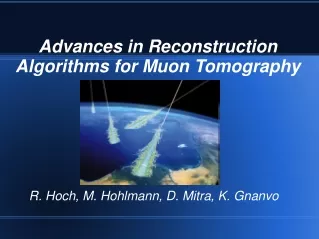
Muon Tomography Algorithms for Nuclear Threat Detection
310 likes | 627 Vues
Muon Tomography Algorithms for Nuclear Threat Detection. R. Hoch, D. Mitra, M. Hohlmann, K. Gnanvo. Tomography. Imaging by sections Image different sides of a volume Use reconstruction algorithms to combine 2D images into 3D Used in many applications Medical Biological Oceanography

Muon Tomography Algorithms for Nuclear Threat Detection
E N D
Presentation Transcript
Muon Tomography Algorithms for Nuclear Threat Detection • R. Hoch, D. Mitra, M. Hohlmann, K. Gnanvo
Tomography • Imaging by sections • Image different sides of a volume • Use reconstruction algorithms to combine 2D images into 3D • Used in many applications • Medical • Biological • Oceanography • Cargo Inspections?
Muons • Cosmic Ray Muons • More massive cousin of electron • Produced by cosmic ray decay • Sea level rate 1 per cm^2/min • Highly penetrating, but affected by Coulomb force
Muon Tomography • Previous work imaged large structures using radiography • Not enough muon loss to image smaller containers • Use multiple coulomb scattering as main criteria
Reconstruction Algorithms • Point of Closest Approach (POCA) • Geometry based • Estimate where muon scattered • Expectation Maximization (EM) • Developed at Los Alamos National Laboratory • More physics based • Uses more information than POCA • Estimate what type of material is in a given sub-volume
Simulations • Geant4 - simulates the passage of particles through matter • CRY – generates cosmic ray shower distributions
POCA Concept Incoming ray 3D POCA Emerging ray
POCA Result 40cmx40cmx20cm Blocks (Al, Fe, Pb, W, U) Unit: mm Θ (degrees) U W Z Pb Fe Al X Y
POCA Discussion • Pro’s • Fast and efficient • Can be updated continuously • Accurate for simple scenario’s • Con’s • Doesn’t use all available information • Unscattered tracks are useless • Performance decreases for complex scenarios
Expectation Maximization • Explained in 1977 paper by Dempster, Laird and Rubin • Finds maximum likelihood estimates of parameters in probabilistic models using “hidden” data • Iteratively alternates between an Expectation (E) and Maximization (M) steps • E-Step computes an expectation of the log likelihood with respect to the current estimate of the distribution for the “hidden” data • M-Step computes the parameters which maximize the expected log likelihood found on the E step
Basic Physics Scattering Angle Scattering function Distribution ~ Gaussian Non-deterministic (Rossi)
EM Concept L T Voxels following POCA track
Algorithm • gather data: (ΔΘx, Δθy, Δx, Δy, pr^2) • estimate LT for all muon-tracks • initialize λ (small non-zero number) • for each iteration k=1 to I • for each muon-track i=1 to M • Compute Cij - E-Step • for each voxel j=1 to N M-Step • return λ
5 40cmx40xcmx20cm Boxes Scenario 1 Geometry
10 minutes exposure 10cmx10cmx10cm voxels Scenario 1 Results Axis in mm Λ (mrad^2/cm) Z X Y
Accuracy Test Scenario 1 Results 48000 total voxels, 32 Uranium Threshhold: 1000 True Positives: 25 False Negatives: 7 True Positive Rate: 78.1% False Positives: 119 False Positive Rate: 0.0025%
Simulated Truck Red Boxes are Uranium Blue are Lower Z Materials Scenario 2 Geometry
10 minutes exposure 5cmx5cmx5cm voxels Scenario 2 Results Axis in mm Λ (mrad^2/cm) Z X Y
Accuracy Test Scenario 2 Results 9704448 total voxels, 106 Uranium Threshhold: 1000 True Positives: 90 False Negatives: 16 True Positive Rate: 85% False Positives: 62 False Positive Rate: 0.000006%
Median Method • Rare large scattering events cause the average correction value to be too big • Instead, use median as opposed to average • Significant computational and storage issues • Use binning to get an approximate median
Aproximate Median Cij= -357,000 Cij = -45,000 Cij = 25,000 Cij = 986,000 Bin Size = 100,000 5 10 20 18 9 11 15 21 23 7 -400,000- -300,000 -200,000 -100,000 0 100,000 200,000 300,000 400,000+ 5 15 35 53 62 73 88 109 132 139 Total Tracks = 139 Median Track at 70 Track 70 in Bin 6 Take Average of Bin 6 (Total Value of Cij's / 11)
Scenario 1 Results 10 minutes exposure 5cmx5cmx5cm voxels Axis in mm Λ (mrad^2/cm) Z X Y
Accuracy Test Scenario 1 Results 48000 total voxels, 32 Uranium Threshhold: 500 True Positives: 26 False Negatives: 6 True Positive Rate: 81.1% False Positives: 31 False Positive Rate: 0.000625%
Scenario 2 Results 10 minutes exposure 5cmx5cmx5cm voxels Axis in mm Λ (mrad^2/cm) Z X Y
Accuracy Test Scenario 2 Results 9704448 total voxels, 106 Uranium Threshhold: 500 True Positives: 97 False Negatives: 9 True Positive Rate: 91.5% False Positives: 5 False Positive Rate: 0.000001%
Future Work • Improvement of absolute lambda values • Real-time EM • Analysis of complex scenarios
Scenario 1: Average Method: 316s Approximate Median Method: 1533s Median Method: ~12hrs Scenario 2: Average Method: 1573s Approximate Median Method: 7953s Median Method: +30hrs Timing
Why Muon Tomography? • Other ways to detect: • Gamma ray detectors (passive and active) • X-Rays • Manual search • Muon Tomography advantages: • Natural source of radiation • Less expensive and less dangerous • Decreased chance of human error • More probing i.e. tougher to shield against • Can detect non-radioactive materials • Potentially quicker searches
