Gas Hydrate Modeling
Gas Hydrate Modeling. by Jack Schuenemeyer Southwest Statistical Consulting, LLC Cortez, Colorado USA 2012 International Association of Mathematical Geoscientists Distinguished Lecturer. Dallas Geophysical Society, March 22, 2012. Thanks to:.

Gas Hydrate Modeling
E N D
Presentation Transcript
Gas Hydrate Modeling by Jack Schuenemeyer Southwest Statistical Consulting, LLC Cortez, Colorado USA 2012 International Association of Mathematical Geoscientists Distinguished Lecturer Dallas Geophysical Society, March 22, 2012
Thanks to: • US Bureau of Ocean and Energy Management (BOEM) for financial support • Matt Frye, BOEM project leader • Tim Collett, US Geological Survey • Gordon Kaufman, MIT, Professor Emeritus • Ray Faith, MIT, retired • Also • This is a work in progress • Opinions expressed are mine
Outline • Purpose of model • Model overview • Generation – some detail • Dependency • A statistician’s perspective
Methane in Ice Courtesy USGS
Location of Hydrates US BOEM
Where are They? USGS
Interest in Hydrates • Governments of: • USA • Japan • India • China • South Korea • Canada • Major energy companies • Universities
Comparison: In-place Hydrates • USGS, 1995 GOM 38,251 tcf • BOEM, 2008 GOM 21,444 tcf • BOEM, 2008 GOM sand only 6,717 tcf • EIA 2011 US Natural gas consumption 24.1 tcf • EIA 2011 US Natural gas production 25.1 tcf
1995 USGS AssessmentSize-Frequency Model Size Frequency
BOEM Mass Balance Model • Cell based model (square 3 to 4 km on a side) • Estimates in-place gas hydrates • Biogenic process (thermogenic omitted) • Stochastic as opposed to scenario • US Federal offshore • Below 300 meters water depth
The Gas Hydrate Assessment Model Basin Under sat Generate HSZ All Cells in Basin Concentration Charge Volume
Input Data for Each Cell(GOM 200,000 cells, 2.32 km2 each) • Location • Water depth • Sediment thickness • Crustal age (Pleistocene to Oligocene) • Fraction sand • Presence of bottom surface reflector • Total organic carbon
Sources of Data • Hard Data • Drilling • Geophysical • Published literature • Analogs • Expert judgment
Model Parameter Inputs • Excel spreadsheet • Specific distribution or regression • Water bottom temp model • Hydrate stability temperature • Phase stability equations • Shale porosity • Sand porosity • Saturation matrix pore volumes
Important Model Variables with a Stochastic Component • Total Organic Carbon (TOC) • Rock Eval (quality measure) • Geothermal gradient (GTG) • Migration efficiency • Undersaturated zone thickness • Sand permeability • Sand and shale porosity • Shallow sand and shale porosities • Water bottom temperature • Formation volume factor
What This Statistician Worries About • Representative data • Model structure • Expert judgment • Uncertainty interval
Look At Models • Generation • Hydrate Stability Zone (HSZ) • Volume
GOM Asymptotic Conversion Efficiency Weibull fit
GOM Geothermal Gradient C0/km of depth Truncated normal fit
Temp/Perm/Porosity • Compute midpoint thickness • Top & bottom temp • Midpt sand perm • Midpt shale porosity • Midpt shale perm • Ave bulk rock perm (i,j); scaled by WB perm
Productivity Function • Generation potential (in grams): • Total Organic Carbon x Asymptotic conversion efficiency x Sediment thickness x Cell area x Sediment density • Incremental Generation from epoch i to j: • Total Organic Carbon x Age duration x Cell area x Intercept x Arrhenius integral / Geothermal gradient
Intercept is a Product of: • Maximum initial production, • Epoch thicknesses, • Seafloor temperature (from model), • Top and bottom temperatures between, epochs fn(thickness and geothermal gradient), • Seafloor perm: function(sand/shale ratio), • Sand & shale permeability
Maximum Initial Production Grams/cubic meter/million years x 106
To Derive Max Initial Production From Price & Sowers, Proc NAS, 2004
Arrhenius’ Law (Deg C)
Estimate Hydrate Stability Zone (HSZ) • HSZ is a zero of: • where • GTG is geothermal gradient (degrees/km) • WBT is water bottom temperature; a function of water depth (WD) Modified from Milkov and Sassen (2001)
Volume • Let X1 = charge (g) at RTP • Let X2 = (X1 x 0.001396) cu m at STP, where 0.001396 = 22.4 liters/mole x (1/(16.0425 g/mole)) / (1000 liters/cu m) converts grams to cubic meters. • Let X3 = X2/fvf (cu m) at RTP, where fvf is the formation volume factor • Let Y = container size (cu m) at RTP = NetHSZ (m) x 30482 (m2) x Saturation • Then if X3 > Y then Vol = Y, else Vol = X3 • Vol <= Vol x fvf
Model Construction • 1st stage • Published literature • Review theory • Review models • Historic data • Identify needs for additional data • Identify experts
Model Construction • 2nd stage • New data • Create flow diagram • Modify existing models • Develop new models • Decide on modeling approach, i.e., Monte Carlo, scenario, deterministic, etc. • Code model
Model Construction • 3rd stage • Run model • Debug model • Run model • Debug model • Run model • Debug model • DOCUMENT • Evaluate model
Model Construction • 3rd, 4th, 5th, … stages • Model results to subject matter experts • Use new data when possible • Revise model • DOCUMENT
A Statistician’s Concerns • Uncertainty • Input data • Model components • Propagation of error • Consistence with knowledge • Bias • Statistical • Sampling • Measurement error
More Concerns • Use of analogs • Expert judgment • Dependency/correlation • Input – model components – aggregation • Spatial correlation • Data/coverage
More Concerns • Hard data • Occasionally data rich – satellite • Usually data poor – drilling expensive • Historical data sometimes unknown quality • Often spatially clustered • “Soft” data – expert opinion • Electing information • Analogs • Integrating hard and soft data
Partial Solutions • Documentation • However … • Evaluation • Results seem reasonable – not all scientific results seem reasonable at first • Consistent with measurements where hard data exists • Make available to public
Dependency Concerns • Many past oil, gas and other resource assessments have assumed: • Pairwise independence between assessment units (plays, cells, basins, etc.) • Total (fractile) dependence