Download
1 / 50
500 likes | 516 Vues
Learn to model transportation systems, solve network flow problems, and optimize operations using prescriptive tools & modeling techniques in this comprehensive new stage course. Explore international aspects, inventory management, and route selection. Benefit from integer answers for free.

E N D
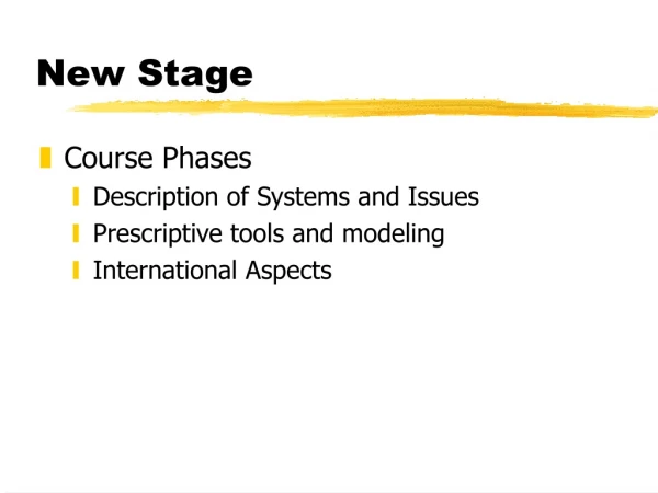
New Stage • Course Phases • Description of Systems and Issues • Prescriptive tools and modeling • International Aspects
Prescriptive Tools & Models • Network Flows • Principally Transportation • Limited direct applications • Good start on modeling • Integer answers for free • Added realism • Weight and cube -- conveyance capacity • Frequency and Schedule Driven systems • Inventory and Load Driven systems • Trailer fill and customer service • Location models • Routing
No Text • There is no text for this portion of the course • Be sure to ask questions in class • Work on your case! The issues in the case parallel those covered in class • Keep up. Attend help sessions with Manu. • The Case is excellent preparation for the exam.
Transportation/Network Models • Single Commodity • Route Selection (Shortest Path) • Basic Network Design (Spanning Tree) • Basic Transportation (Transportation Model) • Cross Docking (Transshipment Models) • Multiple Commodities
Route Selection • Getting From A to B • Underlying Network • Roads • Airports • Telecommunication links • Costs of using each link • Find the cheapest (shortest) path
Example I B E 84 84 90 A 132 138 66 120 C 90 126 H F 60 348 156 126 132 48 J 150 D 48 G Directed Edges
Shortest Path Model • An introduction to AMPL and review of modeling • Sets • Define entities and index data • The Nodes of the Graph • set NODES; • The Edges of the Graph • set EDGES within NODES cross NODES;
Shortest Path Model • Parameters • Hold data • The Cost on each Edge • param Cost{EDGES}; • The Origin and Destination • param Origin symbolic; • param Destination symbolic;
Shortest Path Model • The Variables • The decisions the model should make • Which edges to use • var UseEdge{EDGES} >= 0; • /* The number of times we use each edge */
Shortest Path Model • The Objective • How we distinguish which solution is better • minimize PathCost: • sum{(f,t) in EDGES} Cost[f,t]*UseEdge[f,t];
Shortest Path Model • Constraints • Eliminate what is not feasible • Flow Conservation at each node • s.t. ConserveFlow{node in NODES}: • sum{(f, node) in EDGES} UseEdge[f,node] • - sum{(node, t) in EDGES} UseEdge[node, t] • = (if node = Origin • then -1 • else if node = Destination • then 1 • else 0);
Rules of the Game • To be a linear program • variables can only be of the form • var UseEdge{EDGES} >= lower bound, <= upper bound; • Other possibilities (for later) • var UseEdge{EDGES} binary (meaning 0 or 1) • var UseEdge{EDGES} integer >= 0; • Called Integer Programming
More Rules of the Game • The Objective must be of the form: • minimize ObjectiveName: • sum{(f,t) in EDGES} Cost[f,t]*UseEdge[f,t]; • maximize ObjectiveName: • sum{(f,t) in EDGES} Cost[f,t]*UseEdge[f,t]; • What’s relevant: • minimize or maximize • sum of known constant * variable • What’s not allowed • variable*variable , |variable - constant|, variable2...
More Rules of the Game • The Constraints must be of the form: • s.t ConstraintName: • sum{(f,t) in EDGES} Cost[f,t]*UseEdge[f,t] • <= Constant • s.t. ConstraintName: • sum{(f,t) in EDGES} Cost[f,t]*UseEdge[f,t] • >= Constant • s.t. ConstraintName: • sum{(f,t) in EDGES} Cost[f,t]*UseEdge[f,t] • = Constant
More Rules of the Game • What’s relevant: • Left-hand-side: • sum of known constant * variable • Right-hand-side • known constant • Sense of constraint • >=, <=, = • What’s not allowed • variable*variable , |variable - constant|, variable2...
Network Flow Problems • Special Case of Linear Programs • If the data are integral, the solutions will be integral • Not generally true of Linear Programs, just of Network Flow Problems
To Be a Network Flow Problem • Constraints must be of the form • sum{(f, node) in EDGES} UseEdge[f,node] • - sum{(node, t) in EDGES} UseEdge[node, t] • = or <= or >= constant • And Each variable can appear in at most two constraints, once as a flow in, e.g., as part of the sum sum{(f, node) in EDGES} UseEdge[f,node] once as a flow out, e.g., as part of the sum - sum{(node, t) in EDGES} UseEdge[node, t]
The Data • The Nodes • A named region called Nodes in the spreadsheet d:\personal\3101\ShortPathData.xls table NodesTable IN "ODBC" "d:\personal\3101\ShortPathData.xls" "SQL=SELECT Nodes FROM Nodes": NODES <- [Nodes]; read table NodesTable;
More Data • The Edges and Costs • Named region called Costs table CostsTable IN "ODBC" "d:\personal\3101\ShortPathData.xls" "Costs": EDGES <- [FromNode, ToNode], Cost; read table CostsTable;
More Data • The Origin and Destination • A Named Region called OriginDest table OriginDestTable IN "ODBC" "d:\personal\3101\ShortPathData.xls" "SQL=SELECT Origin, Destination FROM OriginDest": [], Origin, Destination; read table OriginDestTable;
Getting Answers Out table ExportSol OUT "ODBC" "DSN=ShortPathSol" "Solution": {(f,t) in EDGES: UseEdge[f,t] > 0} -> [f~FromNode,t~ToNode], UseEdge[f,t]~UseEdge, UseEdge[f,t]*Cost[f,t]~TotalCost; write table ExportSol;
Running the Model • From a DOS prompt in ..\ilog • Launch AMPL by typing ampl • At the AMPL: prompt type • model d:\….\shortpath.mod; • include d:\…\shortpath.run;
What’s in the .RUN file /* ------------------------------------------------------------------- Read the data -------------------------------------------------------------------*/ read table NodesTable; read table CostsTable; read table OriginDestTable; /* ------------------------------------------------------------------- Solve the problem You may need a command like option solver cplex; -------------------------------------------------------------------*/ solve;
The rest of the .RUN File /* ------------------------------------------------------------------- Write the solution out: May encounter write access error -------------------------------------------------------------------*/ table UseEdgeOutTable OUT "ODBC" "d:\personal\3101\ShortPathData.xls": {(f,t) in EDGES} -> [FromNode, ToNode], UseEdge[f, t]~UseEdge, UseEdge[f,t]*Cost[f,t]~TotalCost; write table UseEdgeOutTable;
Applicability • Single Origin • Single Destination • No requirement to visit intermediate nodes • No “negative cycles” • Answer will always be either • a simple path • infeasible • unbounded
Tree of Shortest Paths • Find shortest paths from Origin to each node • Send n-1 units from origin • Get 1 unit to each destination
Shortest Path Problem Just change the Conservation Constraints... s.t. ConserveFlow{thenode in NODES}: sum{(f, thenode) in EDGES} UseEdge[f, thenode] - sum{(thenode, t) in EDGES} UseEdge[thenode, t] = (if thenode = Origin then -(card(NODES)-1) else 1);
Use Some Care • The Answer is how many paths the edge is in. Not whether or not it is in a path.
Minimum Spanning Tree • Find the cheapest total cost of edges required to tie all the nodes together I B E 84 84 90 A 132 138 66 120 C 90 126 H F 60 348 156 126 132 48 J 150 D 48 G
Greedy Algorithm • Consider links from cheapest to most expensive • Add a link if it does not create a cycle with already chosen links • Reject the link if it creates a cycle.
What’s the difference • Shortest Path Problem • Rider’s version • Consider the number of riders who will use it • Spanning Tree Problem • Builder’s version • Consider only the cost of construction • NOT A NETWORK FLOW PROBLEM
Transportation Problem • Sources with limited supply • Destinations with requirements • Cost proportional to volume • Multiple sourcing allowed
Netherlands Amsterdam 500 * 800 The Hague * Germany 500 Tilburg * 700 * Antwerp Leipzig * Belgium 400 * Liege 200 Nancy * 900 Miles 0 50 100 PROTRAC Engine Distribution 500 800 500 400 700 200 900
Transportation Costs Unit transportation costs from harbors to plants Minimize the transportation costs involved in moving the engines from the harbors to the plants
A Transportation Model • The Sets • The set of Ports set PORTS; • The set of Plants set PLANTS; • The set of Edges is assumed to be all port-plant pairs. If it is not, we should define the set of edges.
A Transportation Model • The Parameters • Supply at the Ports param Supply{PORTS}; • Demand at the Plants param Demand{PLANTS}; • Cost per unit to ship param Cost{PORTS,PLANTS};
Transportation Model • The Variables • How much to ship from each port to each plant var Ship{PORTS, PLANTS} >= 0; • The Objective • Minimize the total cost of shipping minimize TotalCost: sum {port in PORTS, plant in PLANTS} Cost[port, plant]*Ship[port, plant];
Transportation Model • The Constraints • Do not exceed supply at any port s.t. RespectSupply {port in PORTS}: sum{plant in PLANTS} Ship[port, plant] <= Supply[port]; • Meet Demand at each plant s.t. MeetDemand {plant in PLANTS}: sum{port in PORTS} Ship[port, plant] >= Demand[plant];
Observations • If Supply and Demand are integral then the answer Ship will be integral as well. • Single Commodity -- doesn’t matter where it came from. • Proportional Costs.
Crossdocking • 3 plants • 2 distribution centers • 2 customers • Minimize shipping costs • Direct from plant to customer • Via DC
A Transshipment Model • The Sets • The Plants • set PLANTS; • The Distribution Centers • set DCS; • The Customers • set CUSTS;
Transshipment Model • The Set of Edges • We assume all Plant-DC, Plant-Customer, DC-Customer edges are possible. • Convenient to define a set of Edges • set EDGES := (PLANTS cross DCS) union • (PLANTS cross CUSTS) union • (DCS cross CUSTS);
A Transshipment Model • The Parameters • The Supply at each plant • param Supply{PLANTS}; • The Demand at each Customer • param Demand{CUSTS}; • The Cost on each edge. • param Cost{EDGES}; • See the convenience of defining EDGES?
A Transshipment Model • The Variables • The volume shipped on each edge • var Ship{EDGES} >= 0; • The Constraints • Combine ideas of Shortest paths (flow conservation) with Transportation (meet supply and demand)
A Transshipment Model • For each Plant s.t. RespectSupply {plant in PLANTS}: sum{(plant, t) in EDGES} Ship[plant,t] <= Supply[plant]; • For each Customer s.t. MeetDemand {cust in CUSTS}: sum{(f, cust) in EDGES} Ship[f, cust] >= Demand[cust];
A Transshipment Model • For each DC: Conserve flow s.t. ConserveFlow {dc in DCS}: sum{(f, dc) in EDGES} Ship[f,dc] = sum{(dc, t) in EDGES} Ship[dc,t]; • Flow into the DC = Flow out of the DC
Good News • Lots of applications • Simple Model • Optimal Solutions Quickly • Integral Data, Integral Answers
Bad News • What’s Missing? • Single Homogenous Product • Linear Costs • No conversions or losses • ...
Linear Costs • No Fixed Charges • No Volume Discounts • No Economies of Scale