Faster shortest path algorithms for planar graphs
Faster shortest path algorithms for planar graphs. Algorithms seminar 2009 By Ety Khaitsin. Linear time algorithm for single source shortest paths in planar graphs with non-negative lengths. Based on: Separators -> Division -> Recursive division Upgraded Dijkstra.

Faster shortest path algorithms for planar graphs
E N D
Presentation Transcript
Faster shortest path algorithms for planar graphs Algorithms seminar 2009 By Ety Khaitsin
Linear time algorithm for single source shortest paths in planar graphs with non-negative lengths. Based on: Separators -> Division -> Recursive division Upgraded Dijkstra
From Separator to Recursive division f-separator theorem – if any k node graph member of the class has size f(k) separator. (r,s) division -> division into O(n/r) regions. Each region contains at most r nodes, including O(s) boundary nodes. f-separator theorem -> if f(n)=o(n), there is parameter c, such that exists (r, c(f(r)) division for any r. (g,f) recursive division ->contains RG, if |RG|>1 then it contains(g(n), f(g(n))) division of RG, and then recursive division of each region, until the region has only 1 edge. f-separator theorem -> if f(n)=o(n), there is parameter c, such that exists (g,cf) recursive division for any g if g(n)=o(n). Planar graphs closed under √n-separator theorem, then for g:g(n)=o(n), there exists parameter c such that there exists (g,c √n) recursive division in any planar graph
G=(V,E), |V|=n=1300 g(n)=√n , f(n)=√n (g(n), f(g(n))) = (36, 6) There would be O(36) regions, each will contain up to 36 nodes, and each region will have O(6) boundary nodes. RG … … … |R2|≤36 => (g(n), f(g(n))) = (6, 2) There would be O(6) regions, each will contain up to 6 nodes, and each region will have O(2) boundary nodes. |R1|≤6 => (g(n), f(g(n))) = (2, 1) There would be only atomic regions R(u,v) which contains a single edge (u,v)
Simplified algorithm Simplified algorithm will run O(n log log (n)) and will use the same techniques of the main algorithm. Divide graph into regions, each of size , containing boundary nodes. Initiation: all nodes labels ∞, all edges deactivated set d(s)=0, activate outgoing s edges. Algorithm: while(true) 1. Select region containing lowest label node that has active outgoing edge in the region. 2.repeat (log n) times: 2A. select lowest labeled node with outgoing activated edge in the region. Relax and deactivate all outgoing edges to this region. Relax all outgoing edges (v,w) to other regions and if decreased d(w) activate w outgoing edges.
Analyze it… Dijkstra on region would repeat |R(V)| times: • every node selected exactly once • too expensive in run time – this region will be selected again Distances are not correct while doing one region -> don’t spend too much time in 2A. Making less times Step1 -> “charge” each Step 1 with enough Step 2A iterations Charge Step1 with log(n) Step 2A iterations. No active outgoing edges – iteration truncated. Doesn’t mean this region wouldn’t iterated again, can be waked up after relaxing edge from other region to boundary node of this region. Relatively few boundary nodes – few truncated iterations
Back to multilevel algorithm Atomic region has only one edge – R(u,v) Level– level of atomic region = 0 level of non atomic region = max level of children + 1 Label – d(v) for each node Priority queue – Q(R) of each region, contains immediate children regions. Q(R) of atomic region R contains the edge itself (the key in this case would be label of the tail or ∞)
Initiation All labels := ∞ All keys in all queues := ∞ d(s) := 0 for each outgoing edge of s - (s,v): GlobalUpdate(R(s,v), (s,v), 0) Activate(RG)
Activate(R) A1 if R atomic on (u,v): A2 if d(v) > d(u) + len(u,v) then d(v) := d(u) + len(u,v) for each outgoing edge (v,w): GlobalUpdate(R(v,w), (v,w), d(v)) A3 updateKey(Q(R), (u,v), ∞) A4 return minKey(Q(R)) A5 else A6 repeat αlevel (R)times OR until minKey(Q(R)) = ∞ : A7 R’ := minItem(Q(R)) A8 k := Activate(R’), updateKey(Q(R), R’, k) A9 return minKey(Q(R)) GlobalUpdate(R, x, k) G1 updateKey(Q(R), x, k) G2 if minKey(Q(R)) changed: G3 GlobalUpdate(parent(R), R, k)
RG Key=0 s
Correctness Easy to see that if : • d(s) = 0 • d(v) is upper bound on distance from s to v • every edge is relaxed edge (u,v) is relaxed if d(v) <= d(u) + len(u,v) then labels d(v) gives correct distances. 1. d(s) = 0 : initiation 2. d(v) is upper bound on distance from s to v : induction on algorithm steps: initially all ∞ d(v) changes at A2: d(v) := d(u) + len(u,v) d(u) – inductively upper bound
Lets prove that all edges are relaxed… Pending edge (u,v) – if the key of (u,v) in Q(R(u,v,) is finite. Lemma 3.2: If edge (u,v) is not pending, it is relaxed Initially – all pending become pending at A3 -> after edge is relaxed become unrelaxed when d(v) or d(u) change -> when d(u) reduced in A2 on (w,u) -> call GlobalUpdate to all (u,v) -> makes edge pending Lemma 3.3: The key of pending edge (v,w) is d(v) Initially – all keys are ∞ d(v) changes only at A2 or initialization (v=s) -> call GlobalUpdate on all outgoing edges (v,w) with key d(v)
current invocation – invocation of activate function current region– region that current invocation applied on Lemma 3.4: If R not ancestor of current region then key of R in Q(parent(R)) = minKey(Q(R)) Initially – all keys are ∞ if minKey(Q(R)) changed at GlobalUpdate -> at G3 the key of R in Q(Parent(R)) will be updated to this minimum. when new Activate invoked -> applies to less regions -> still holds when Activate(R) returns -> key of R in parent’s queue updated to minKey(Q(R)) strictly after Activate(R) ends Lemma 3.5: If R not ancestor of current region then minKey(Q(R)) = min{ d(v) | (v,w) is pending edge in R } induction on level(R): in atomic region R(v,w) key is always ∞ or d(v) (lemma 3.3) for not atomic region – inductively using 3.4 lemma
3. all edges are relaxed… Algorithm should terminate after minKey(Q(RG)) = ∞ assign: αlevel(RG) = ∞ by Lemma 3.5 : minKey(Q(RG))= ∞ -> all edges are not pending by Lemma 3.2: all edges are not pending -> all edges relaxed when algorithm terminates, all edges relaxed -> for each node v: d(v) = distance(s,v)
Analysis Linear ≠ Trivial Depend on (g,f)-recursive division, and αiparameters. f(n) ≈ √n , g(n) ≈ The division itself is linear for planar graphs. Assumes every node v has: din(v) ≤ 2, dout(v) ≤ 2
Intuition Algorithm using steps like Dijkstra, but it jumps from one region to another to reduce the cost – spend more time in smaller regions which have smaller queues. There is a tradeoff: If jumps from one region to other would be too often, more heavy operations on bigger queues will be performed. If doing many iterations in the regions – those iterations may be lost because the distances not correct.
We wish to charge every iteration on region i, with αi-1 of iteration on region i-1. If the invocation of Active ends before it makes αi-1 iterations we call it truncated activation. Truncated execution is not definitely the final execution on this region. An edge from other region to node in this one, can change it’s label, and then make all it’s outgoing edges pending. This will cause new invocation on this region. We bound number of such “Wakes up” using the fact that it always caused by boundary node of this region, and each region have few boundary nodes.
Central player – Activate invocation A is Activate invocation on region R: level(A) – level(R) start key (A) – minKey(Q(R)) when A begins end key (A) – minKey(Q(R)) after A ends start node (A) – when A begins, the node v: d(v) = minKey(Q(R)) = min{d(v)|(v,w) is pending edge in R} = key of R in parent(R) if A invoke B -> B child of A partial order ≤ : A ≤ B if both invoked on same region R, and A before B
truncated invocation A – if end key(A) = ∞ - every invocation on atomic region is truncated entry node of region R – boundary node of R, which has outgoing edge inside R. • s is entry node of RG • example: u is entry node of R(u,v) every truncated invocation A, charged to pair (R,v), when R is ancestor of A’s region and v is entry node of R Charging scheme invariant: For any pair (R,v) there is invocation B on R, such that all chargers of (R,v) are descendents of B.
Lets bound number of chargers (R,v): Let i be level of R, and let j>i, count level j chargers: All of them descendents of invocation B on R. B is only charger of level i, B has at most αi children, each has αi-1children etc. Number of descendents of B at level j is ( , ) Lemma: For level-i region R and entry node v of R, pair (R,v) has at most level j chargers.
Simple algorithm analysis In simple algorithm we have α1=log(n), α2=1 We will prove it takes O(n*loglog(n)) time using all analysis steps used in main algorithm analysis. Bound number of chargers for any pair (R,v) : • L(R)=0 : (R,v) charged by at most 1 level-0 invocation. • L(R)=1: at most 1 level-1 invocation and α1level-0 invocations. • L(R)=2: at most 1 level-2, α2=1 level-1 and α1 level-0 invocations.
Now we bound number of such pairs: • L(R)=0 : O(n) pairs (|E|=O(n)) , at most O(n) truncated L-0 invocations charged by L-0 regions. • L(R)=1: L-1 regions, each has boundary nodes, so there pairs, each has at most log(n) L-0 chargers, total chargers: • Level(R)=2: 1 pair (RG,s), charged by log(n) L-0 invocations. -> there O(n) L-0 truncated invocations -> in similar way: L-1 truncated invocations -> and 1 L-2 truncated invocation
Let Si be number of Level-i invocations (truncated & not truncated): S0 = O(n) – because all invocations truncated Level-j not truncated invocation creates αj Level-(j-1) invocations -> S’j (not truncated) = S(j-1)/ αj S1 ≤ S0/α1 + = O(n/log(n)) S2 ≤ S1/ α2 + 1 = S1+1 = O(n/log(n)) Now we bound the time Ti of L-i invocation (without recursion and GlobalUpdate): T0 = O(1). T1 = log(n) operations on queue of size , each operation O(loglog(n)) = O(log(n)*loglog(n)) T2 = 1 operation on queue of size , so T2=O(log(n)) Total time without GlobalUpdate =
Analyze time spent in Global Update: • every atomic region R(u,v) can start up to 2 calls of GlobalUpdate - dout(v) ≤ 2 . • recursive call: R(u,v)=R0,…,Rp p≤2 (Ri parent of Ri-1) • Queue operation time: • Q(R0) = O(1), • Q(R1) = O(loglog(n)) • Q(R2)=O(log(n)) -> if p<2: then GlobalUpdate takes up to O(loglog(n)) time -> there O(n) atomic regions at all, all GlobalUpdate which recursion stops before R2=RG (p<2) takes O(n*loglog(n)).
Level-0 invocations are charged to: • type1: Level-1 or Level-2 regions, there O(n/log(n)) those invocations and there total time is O(n*log(n)/log(n)) = O(n) • type2: Level-0 regions: each such invocation on R(uv) associated with node which label changed – v. din(v) ≤ 2 then at most 2 L-0 invocations associated with v. p=2 -> v is entry node of Level-1 region. Total entry nodes for Level-1 regions, then there level-0 invocations charged on level-0 regions and p=2: their total time is O(n/log(n)) All those cases show that total time of algorithm is O(n*loglog(n))
Multilevel analysis steps… • Check the changes at value minKey(Q(R)) – while an Activate(R) runs: • How it is changes when other Activates invoked during current invocation? • How it is changed, from one invocation to other on the same region? • When minKey(Q(R)) stops reducing – it means the region already has it minimal value – happens at stable invocation. • Changing of minimal keys is depends at start nodes of invocation – if it is an entry node or not.
Chargee of truncated invocation A on R –> (v,R’) (region and start node of entryPred(stableAnc(A)) ) • stableAnc(A) - First invocation A’ on R’, ancestor of A that is stable – minKey(Q(R)) never reduced again • R’ is a ancestor of R, v is the entry node of R’ • entryPred (A’)- First invocation E before A’ on R’ that started at entry node • v is the entry node of R • Prove the Charging scheme invariant • Calculate the time analysis – steps like in simple algorithm analysis
Lemma 3.6: A invocation on R, A’ child of A. start key (A’) = minKey(Q(R)) when A’ starts A’ invoked on R’ -> R’ = minItem(Q(R)) -> by lemma 3.4: key of R’ in Q(R) = minKey(Q(R’)) = start key (A’) Lemma 3.7: (1) during invocation A, every key assigned ≥ start key (A) (2) A1, A2, … Ap children of A ordered by start time then: start(A)=start(A1) start(A1) ≤ start(A2) ≤ … ≤ start(Ap) start(Ap) ≤ end(A) Induction on level(A) base: R(u,v) -> GlobalUpdate with key d(u)+len(u,v) >= d(u) = start key(R(u,v)) i=1..p:ki = minKey(Q(R)) when Ai starts, kp+1 = minKey(Q(R)) when Ap ends using lemma 3.6 and induction on (1) prove: ki+1>ki
Lemma 3.8: Let k be key associated with R at some time t, A first invocation on R after t. If start(A) < k then A starts at entry node. • some edge uv key decreased between t and A invocation • A is first invocation – decrease in GlobalUpdate during initialization or Activate – both mean u is entry node of R. Lemma 3.9: Let A and B be invocations on R, B immediate after A. if end(A)>start(B) then B starts with an entry node. • k=end(A) Lemma 3.10: For each region R, first invocation with region R starts with entry node. • t = moment before initialization
Lemma 3.11: if A<B two invocations with same start node v, then start(A) > start(B) After A ends, outgoing edges of v are relaxed (the first relaxed regions). B start at v, means some edge vu pending again -> d(v) was reduced. Lemma 3.12: for every invocation A, start(A) >= start(entryPred(A)) by 3.9 – otherwise A should start at entry node
Lemma 3.13: A<B such that enteryPred(A)=enteryPred(B). If B is stable, then every child of A is stable. enteryPred(A)<A<C0<…Ci...<Cp=B<Cp+1<… A’ < C’ A’ stable -> start(A’) <= start(C’) by 3.9: i<=p end(Ci-1)<=start(Ci) / Cidoesn’t start at entry node (*) by 3.7 : start(Ci)<= start(C’) /children invocation lemma start(A’)<=end(A) need to show : end(A)<= start(Ci) • i<=p : by (*) • i>p: Ci>B and B stable then: start(Ci)≥start(B) and start(B) ≥ end(A) by (*) -> end(A) ≤ start(Ci)
Charging scheme invariant: For each pair (R,v) there is an invocation A on R such that every charger of (R,v) is decsendant of A. A=stableAnc(C), E=enteryPred(A) RG E <= A < B : on R, E has start node v. C C’ : A is the earliest invocation that has a charger C show that no C’ cannot be the charger of (R,v) Suppose not, Let E’ = enteryPred(B): if E < E’ : E ≤ A<E’≤B -> start(E)<start(E’) (start at same node v) -> start(E’)<start(A) (contradiction to stable(A)) -> E=enteryPred(B) • C=A: let A’ : E ≤ A < A’ ≤ B, A is charger then truncated, then A’ start at entry node, contradiction to E=enteryPred(B). • C ≠A: B = stableAnc(C’) -> C is stable -> C=stableAnc(C), contradiction to A=stableAnc(C).